Magnetic moment of an electron (NLO)

In this section we derive the next-to-leading-order (NLO) order-$\alpha^2$ correction to the magnetic moment of an electron. This has been first attempted in 1950 by Karplus and Kroll, and first computed correctly in 1957 by Petermann and Sommerfield.

See for example hep-ph/9410248 for the expression for $A_2$:

Code:

>>> from sympy import zeta, S, log
>>> A_2 = S(197)/144 + zeta(2)/2 + 3*zeta(3)/4 - 3*zeta(2) * log(2)
>>> A_2.n()
-0.328478965579194

Plan of the calculation¶

Status: all five contributions reproduced. Each gets its own section below: the diagram, whether/how it must be renormalized, the computation strategy, the known analytic value, and our own SymPy derivation cross-checked numerically in Fortran. Diagrams IIe, IId, IIc and IIa are established analytically (with the hardest pieces of IIc and IIa identified from 11–14-digit quad-precision integrals), diagram I is confirmed numerically, and pixi run assembly proves in SymPy that the five values sum to $A_2$ with the infrared logarithms cancelling.

As in the LO section, the anomalous moment is the on-shell form factor

now evaluated to order $\alpha^2$: we must compute the two-loop (fourth-order in $e$) contributions to the vertex function $\Gamma^\mu(p', p)$, project out $F_2$, and take $q^2 \to 0$.

Papers (all in this repo)¶

• twoloop.pdf — R. Karplus and N. M. Kroll, Phys. Rev. 77 (1950) 536 (“KK”). The first attempt; defines the diagram classification I, IIa–IIf used by all the 1950s papers (their Fig. 1). Their values for diagrams I and IIc were wrong.

• petermann1957.pdf — A. Petermann, Helv. Phys. Acta 30 (1957) 407. The full analytic evaluation of the five independent contributions; our per-diagram reference values (eqs. (1)–(6)) are from this paper.

• petermann1958.pdf — A. Petermann, Nucl. Phys. 5 (1958) 677. Rigorous upper/lower bounds proving KK’s $\mu_{\mathrm{IIc}}$ wrong; gives the complete auxiliary-variable integrands for IIc (his eqs. (2.1)–(2.4)) — our reproduction target for that diagram.

• sommerfield1957.pdf — C. M. Sommerfield, Phys. Rev. 107 (1957) 328; sommerfield1958.pdf — Ann. Phys. 5 (1958) 26. Independent calculation by Schwinger’s mass-operator method, confirming Petermann’s total.

• laporta1991.pdf, laporta1993.pdf, laporta1994.pdf — S. Laporta (with E. Remiddi in 1991): analytic values of sixth-order (three-loop) graphs. Not needed for $A_2$; kept for the later $A_3$ project.

The Karplus–Kroll diagram classification¶

KK’s Fig. 1 groups the fourth-order diagrams for electron scattering off an external field into five classes:

• Class I — the crossed-ladder (“irreducible”) vertex diagram.

• Class II (a–f) — the “reducible” two-loop vertex diagrams: they contain a one-loop subdiagram (vertex part, self-energy, or vacuum polarization) inserted into the LO vertex diagram.

• Class III — vacuum-polarization corrections to the external field line (including light-by-light-type blobs attached to the external potential). These modify the external potential, not the electron’s moment: no contribution here. (The light-by-light vertex graphs that do contribute to $a_e$ first appear at sixth order — see laporta1991.pdf.)

• Class IV — diagrams reducible to a photon self-energy correction of the scattered wave: pure charge renormalization, no moment contribution.

• Class V — electron-loop tadpole-like diagrams: the two orientations cancel exactly by Furry’s theorem.

So only class I and class II contribute. Within class II, IIb and IIf are self-energy corrections on the external electron legs — pure mass/field renormalization with no moment contribution (see below). The mirror images (reflection through the external vertex) of IIc and IId are not drawn by KK; their contribution is included by doubling. That leaves five independent contributions: I, IIa, IIc, IId, IIe.

Reference values (Petermann 1957)¶

In units of $\alpha^2/\pi^2$, with the photon-mass IR regulator $\lambda$ (petermann1957.pdf, eqs. (1)–(6)):

The infrared logarithms cancel between IIc and IId, and the sum is exactly $A_2$:

>>> from sympy import Rational, pi, zeta, log, symbols, simplify, expand
>>> L = symbols("L")   # L = log(lambda^2/m^2)
>>> mu_I   = Rational(1,6) + Rational(13,36)*pi**2 + Rational(5,4)*zeta(3) \
...          - Rational(5,6)*pi**2*log(2)
>>> mu_IIa = Rational(11,48) + pi**2/18
>>> mu_IIc = -Rational(67,24) + pi**2/18 - zeta(3)/2 + pi**2*log(2)/3 - L/2
>>> mu_IId = Rational(11,24) - pi**2/18 + L/2
>>> mu_IIe = Rational(119,36) - pi**2/3
>>> expand(mu_I + mu_IIa + mu_IIc + mu_IId + mu_IIe)
-pi**2*log(2)/2 + pi**2/12 + 3*zeta(3)/4 + 197/144

For the record, KK’s two errors: their $\mu_\mathrm{I}$ was too low by $\frac{1}{32}$, and their $\mu_\mathrm{IIc} = -3.18$ was too low by

which is how they arrived at the wrong total -2.973.

Caveat on per-diagram comparisons: the split of $A_2$ into the five $\mu$’s is scheme-dependent — it depends on how the UV subtractions (mass, vertex, charge renormalization) are apportioned among the diagrams, and on the IR regulator. To reproduce Petermann’s individual numbers we must follow the KK subtraction conventions (they renormalize each reducible diagram by subtracting the corresponding lower-order renormalization part, which is why e.g. the ladder IIa comes out UV- and IR-finite). Only the total is scheme-independent.

Conventions, regulators, renormalization¶

We keep the conventions of the LO section (Peskin–Schroeder-style, metric $(+,-,-,-)$), with:

• IR: photon mass $\lambda$ (as in KK/Petermann).

• UV: Pauli–Villars, to match the 1950s papers. (A dimensional- regularization pass can be added later as an independent check.)

• electron mass $m = 1$ in all integrals below.

Note that KK/Petermann use the old “Pauli metric” conventions ($i\gamma p + m$ propagators), so a translation is needed when comparing intermediate formulas.

Renormalization structure at this order:

• Mass renormalization: the self-energy subgraph in IId is UV divergent; the on-shell counterterm $\delta m$ (order $\alpha$) is inserted into the internal electron propagators of the LO vertex and subtracted together with IId (“reduced diagram” bookkeeping of KK).

• Vertex renormalization cross term: IIa and IIc contain a divergent one-loop vertex subgraph. As in the LO section we renormalize so that $F_1(0) = 1$ to all orders; writing the unrenormalized $F_1(0) = 1 + \delta F_1(0) + O(\alpha^2)$, the vertex rescaling by $Z_1 = 1 - \delta F_1(0) + \dots$ produces the cross term

  $$-\,\delta F_1(0)\, F_2^{(2)}(0) = -\,\delta F_1(0)\,\frac{\alpha}{2\pi},$$

  (10)

  whose UV part cancels the vertex subdivergences of IIa + IIc and whose $\log\lambda$ part participates in the IR cancellations.

• Wavefunction renormalization $Z_2$ of the external legs: cancels against $Z_1$ by the Ward identity ($Z_1 = Z_2$); equivalently, diagrams IIb/IIf plus the external-leg counterterms give zero moment contribution.

• Charge renormalization: contained in using the once-subtracted vacuum polarization $\hat\Pi(q^2)$ (with $\hat\Pi(0)=0$) in diagram IIe, with $\alpha$ the physical fine-structure constant.

Master strategy for each diagram:

1. Write the amplitude from the Feynman rules (as in the LO section).

2. Project out $F_2(0)$ (magnetic projector / trace technique, so the whole computation reduces to Dirac traces and scalar integrals — done in SymPy).

3. Combine denominators with Feynman parameters, do both loop-momentum integrations, leaving a multi-dimensional parametric integral.

4. Evaluate: numerically first (Fortran, Gauss–Legendre / adaptive quadrature, compiled with flang -O3 -march=native -ffast-math), then analytically in SymPy by sequential one-variable integration in a well-chosen order (this is where $\zeta(3)$, $\pi^2\log 2$, $\pi^2$ arise, exactly as in Petermann’s hand calculation).

Tooling (see pixi.toml tasks): pixi run figures regenerates the diagram SVGs (code/feynman_diagrams.py); pixi run lo-sympy, pixi run lo-trace-sympy, pixi run iie-sympy, pixi run iid-sympy run the SymPy derivations; pixi run iie-fortran, pixi run iid-fortran compile and run the Fortran checks; pixi run g2-nlo runs the fast ones.

A SymPy practicality discovered on the way, used throughout: definite integrate() with a free parameter in the integrand is slow and sometimes wrong (branch issues) — e.g. it returns $\frac12 - r$ for the massive photon kernel $K$ below, which is false. We therefore rationalize all square roots by substitution, take indefinite antiderivatives of partial-fractioned integrands, and evaluate the endpoint limits ourselves, checking every intermediate result numerically.

The pipeline (Dirac algebra, projector, loop integrals)¶

All diagrams are computed by one mechanical pipeline (code/dirac.py, code/loops.py):

• Explicit Dirac algebra: 4×4 gamma matrices in the Dirac representation, explicit on-shell spinors, and explicit Breit-frame kinematics $p = (E, 0, 0, w)$, $p' = (E, 0, 0, -w)$, $q = (0,0,0,-2w)$, $q^2 = -4w^2$ — no abstract index gymnastics, every step is a scalar polynomial identity that can be checked numerically.

• Form-factor projection: sandwiching $\Gamma^\mu$ between explicit spinors and matching against $\gamma^\mu F_1 + i\sigma^{\mu\nu}q_\nu F_2/2m$. The $\mu = 1$ spin-flip sandwich alone measures only the magnetic combination $F_1 + F_2$ (its two basis values coincide), so it is paired with the $\mu = 0$ no-flip sandwich; at $q^2 \to 0$,

  $$F_2(0) = -\tfrac12\left(A_0\big|_{w=0} + \partial_w A_1\big|_{w=0}\right), \qquad A_\mu = \bar u(p')\,\Gamma^\mu\, u(p).$$

  (11)

• Loop integration: Feynman parametrization with automatic completion of the square (feynman_shift), angular averaging of loop momenta at the component level (symmetrize), and a table of $\int \mathrm{d}^4 l\, (l^2)^a/(l^2-\Delta)^n$ with the log-divergent cases carried as an explicit symbol $L_{UV} = \log\Lambda^2$ (Pauli–Villars) — every $F_2$ must be free of $L_{UV}$, which is asserted.

Validation (pixi run lo-trace-sympy, code/g2_lo_trace.py): the whole LO derivation from raw Feynman rules runs through the pipeline and reproduces both Schwinger’s result and the massive-photon kernel:

Delta = -lam**2*y - lam**2*z + lam**2 + m**2*y**2 + 2*m**2*y*z + m**2*z**2   (at q^2 = 0)
UV structure OK: LUV in F1 only
F2 integrand (q^2=0, m=1): -e2*(y + z)*(y + z - 1)/(4*pi**2*(-lam**2*y - lam**2*z + lam**2 + y**2 + 2*y*z + z**2))
F2(0) = 2 * e2/(16 pi^2)  =>  a_e = alpha/(2 pi): True
K(8) from trace pipeline = 0.027280670780387366
K(8) direct              = 0.027280670780387367247
OK: massive-photon kernel reproduced

(The parametric integrand looks different from the LO section because the Feynman parameters are assigned to different propagators, but it integrates to the same kernel.)

Stage 0: LO vertex with a massive photon¶

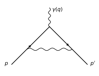
The pipeline is validated on the LO diagram, generalized to a photon of mass $\lambda$ (needed both as the IR regulator and as the spectral mass in diagram IIe). Repeating the LO derivation with $\Delta = (1-z)^2 m^2 - q^2 xy + z\lambda^2$ gives, with $t = \lambda^2/m^2$:

For $t > 4$ (the spectral region needed below) the denominator factors rationally under the substitution

Running pixi run lo-sympy (code/g2_lo.py):

K(0) = 1/2  => a_e = alpha/(2 pi)
K(y) = (-y**2*(y - 1)*(2*y + 3) - 2*y*(y - 1)
        + log(((y + 1)/y)**(2*y**4*(y + 1))*(y + 1)**(-2*y - 2)))
       /(2*y**2*(y - 1))
K(t=8) direct  = 0.02728067078038736724734729
K(t=8) closed  = 0.02728067078038736724734729
OK: closed form matches numeric integration

Diagram IIe: vacuum polarization insertion — DONE¶

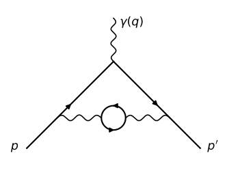
Topology: the LO vertex diagram with the internal photon corrected by an electron loop.

Renormalization: the electron loop $\Pi^{\mu\nu}$ is UV divergent; the once-subtracted $\hat\Pi$ ($\hat\Pi(0) = 0$, i.e. on-shell charge renormalization) makes the diagram finite. It is also IR finite — no $\log\lambda$ — so it is a well-defined number all by itself.

Method (dispersion relation): the renormalized VP gives the spectral representation of the dressed photon propagator,

i.e. diagram IIe is the LO diagram with a massive photon folded with $\rho$:

With $t = (1+y)^2/y$ everything rationalizes ($\sqrt{t(t-4)} = (1-y^2)/y$, $|\mathrm{d}t/\mathrm{d}y| = (1-y^2)/y^2$):

The $y$-integration (rational) is done first; the remaining $z$-integrand is of the form $A(z)\log z + B(z)$ with rational $A, B$, whose integral produces dilogarithms at unit argument, i.e. $\pi^2$.

Result — pixi run iie-sympy (code/g2_iie.py):

after y-integration:
  I(z) = z*(-5*z**3 + 27*z**2 - 27*z + log(z**(3*z**3 - 9*z**2 - 9*z + 3)) + 5)
         /(9*(z**3 - 3*z**2 + 3*z - 1))
mu_IIe = 119/36 - pi**2/3
       = 0.015687421859102682611
OK: mu_IIe = 119/36 - pi^2/3  (Petermann 1957, eq. (5))

Numeric check — pixi run iie-fortran (code/g2_iie.f90, independent 128-point Gauss–Legendre quadrature in the original $t$-form variables):

mu_IIe (numeric)      =    0.015687421859103
119/36 - pi^2/3       =    0.015687421859103
difference            =   2.98E-16

in agreement with petermann1957.pdf, eq. (5).

Diagram IId: self-energy insertion on the internal electron line — DONE¶

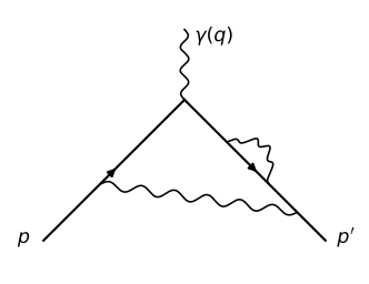
Topology: the LO vertex diagram with the one-loop electron self-energy $\Sigma(p)$ inserted on one internal electron propagator. The mirror diagram contributes equally; $\mu_\mathrm{IId}$ includes both (factor 2).

Renormalization: $\Sigma$ is UV divergent; we use the fully on-shell-subtracted

which is equivalent to adding the $\delta m$-insertion counterterm diagram

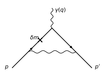
and the $\delta Z_2$ piece. The on-shell subtraction is IR sensitive: $\mu_\mathrm{IId}$ keeps a $+\frac12\log(\lambda^2/m^2)$ that cancels against IIc. The numerical agreement below confirms that this full on-shell subtraction is the KK/Petermann scheme for IId.

Derivation (pixi run iid-sympy, code/g2_iid.py): the pipeline derives the inner loop mechanically,

with $u \in (0,1)$ the inner Feynman parameter. After the on-shell subtraction $L_{UV}$ cancels identically (asserted by the script), leaving a rational part and a $\log\!\big(D_\mathrm{in}(k^2)/D_\mathrm{in}(m^2)\big)$ part. The log is made rational with one more parameter, $\log(X/Y) = \int_0^1 \mathrm{d}\xi\, (X-Y)/(Y + \xi(X-Y))$, which cancels one power of the doubled propagator $(k^2-m^2)^2$ and leaves a normal propagator of mass$^2$ $C = m^2 + (a - b m^2)/(\xi b) > m^2$ (kept as an opaque symbol during assembly to keep expressions small). The outer loop then runs through the same machinery as LO, giving

with $f_\mathrm{rat}$ printed by the script and $f_\mathrm{log}$ (a 65-term rational expression) written, together with $f_\mathrm{rat}$, as generated Fortran into code/g2_iid_frat.inc / code/g2_iid_flog.inc.

Numeric check — pixi run iid-fortran (code/g2_iid.f90, Gauss–Legendre with a smoothstep endpoint map to resolve the IR structure at parameter scale $\lambda$; compile with -fopenmp for speed):

   lam     mu_IId - log(lam)    target = -0.0899780...
  0.1000      0.304059789767   (rat =  -1.4642459, log =  -0.5342794)
  0.0300      0.144669264714   (rat =  -2.7824431, log =  -0.5794456)
  0.0100      0.025773149821   (rat =  -3.9913265, log =  -0.5880705)
  0.0030     -0.043148094904   (rat =  -5.2625440, log =  -0.5897471)
  0.0010     -0.070807985164   (rat =  -6.3885840, log =  -0.5899793)
  0.0003     -0.083100856528   (rat =  -7.6048118, log =  -0.5900172)
extrapolated lam->0:      -0.090070136381
target 11/24-pi^2/18:     -0.089978022283

The $\lambda \to 0$ extrapolation (fitting $c_0 + c_1\lambda + c_2\lambda\log\lambda$ to the three smallest $\lambda$) agrees with Petermann’s constant to 10^-4, and the $\log\lambda$ coefficient is confirmed to be $+\frac12\log\lambda^2$ (subtracted in the table).

Analytic evaluation (pixi run iid-analytic, code/g2_iid_analytic.py, using the deterministic rational-function integrator code/ratint.py, since SymPy’s integrate with symbolic parameters returns wrong results for exactly these integrals):

• The rational piece factorizes: $f_\mathrm{rat} = U'(u)\, S'(y,z)$, with the $(y,z)$-dependence only through $s = y+z$ (times $z$), so $\mu_\mathrm{rat}(\lambda) = U(\lambda) S(\lambda)$ with

  $$U = \int_0^1 \frac{2u(u-2)(u-1)}{(1-u)^2 + \lambda^2 u}\,\mathrm{d}u, \qquad S = \int_0^1 \frac{\tfrac{s^2}{2}(s-1)\left(3s^3+s^2 - \lambda^2(4s-1)(s-1)\right)}{(s^2 + (1-s)\lambda^2)^2}\, \mathrm{d}s,$$

  (21)

  both exact in $\lambda$; the product expands to $\mu_\mathrm{rat} = \log\lambda + \frac12 + O(\lambda)$.

• The log piece is finite at $\lambda = 0$. Its parameter $\xi$ is traded for the spectral mass $C$ ($\mathrm{d}\xi/\xi = -\mathrm{d}C/(C-1)$, $C \in (1/u, \infty)$), and the remaining integrals are done in the order $z$ (polynomial), $C$ (rational), $t$, $s$ (rational-times-log, stays elementary — no dilogarithms until the very last step), $u$. The result is

  $$\mu_\mathrm{log} = -\frac{1}{24} - \frac{\pi^2}{18}.$$

  (22)

Output:

[   0.7s] f_rat factorized form verified
[   1.3s] U, S exact in lam, checked numerically
  mu_rat(lam->0) = log(lam) + 1/2
[   1.9s] z-integration done
[   2.1s] C-integration done, checked numerically
[   3.3s] t-integration done, checked numerically
[   4.0s] s-integration done, checked numerically
[   4.8s] u-integration done, checked numerically
  mu_log(lam=0) = -pi**2/18 - 1/24

mu_IId = 11/24 - pi^2/18 + (1/2) log(lam^2)
      == 11/24 - pi^2/18 + (1/2) log(lam^2/m^2)
      (Petermann 1957, eq. (4));  constant = -0.08997802228274214

in exact agreement with petermann1957.pdf, eq. (4).

Diagram IIa: ladder (vertex part at the external vertex) — DONE¶

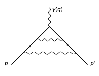
Topology: both photons span the external vertex, nested: the inner photon is a one-loop vertex correction at the external-field vertex.

Renormalization: the inner vertex subgraph is log-divergent; in the KK scheme one subtracts the corresponding second-order renormalization part (the $\delta F_1(0)\,\gamma^\mu$ counterterm) within the diagram, which is what makes their $\mu_\mathrm{IIa}$ UV finite and even IR finite.

Target: $\mu_\mathrm{IIa} = \frac{11}{48} + \frac{\pi^2}{18}$.

Derivation (pixi run iia-sympy, code/g2_iia.py): the same three-piece decomposition as IIc — the inner vertex subgraph (now sitting at the external vertex, so the external momentum $q$ flows through the inner loop), subtracted pointwise in the inner Feynman parameters $(u, v)$ by the on-shell $L_a(u,v)\gamma^\nu$ counterterm whose $(u,v)$-integral is $\delta F_1(0)$; no mirror factor (the ladder is its own mirror image). $L_{UV}$ cancels pointwise (asserted). The three pieces reduce to functions of $s = y{+}z$, $\chi = u{+}v$, $t$, and the $\xi$ of the log-ratio representation only.

Piece (b) (the $\delta F_1 \times$ LO cross term) is exactly half of IIc’s (same factorized integrals, no mirror doubling):

Piece (c) (code/g2_iia_cq.f90): the $\xi$ and $\chi$ integrations are exact (shared letter alphabet with IIc); the remaining 2-dim quad-precision DE quadrature with a $t$-sliver $\delta$-cut and pure-$\delta^2$ Richardson gives, at DE levels 6 and 7,

level  6: C0 (Richardson) =    -0.062500000001992...
level  7: C0 (Richardson) =    -0.062500000006245...

i.e. $C_0 = -\frac{1}{16}$ exactly (11 digits).

Piece (a) (code/g2_iia_a3.f90): the $z$ and $\chi$ integrations are exact, leaving a compact rational 3-dim integrand $s\chi\,g(s,\chi,t)$ (739 ops — far cheaper than emitting the dilog-heavy fully-integrated form). The quad-precision DE ladder in the photon mass, with $V(\lambda) = I(\lambda) - \frac12\log\lambda$ (values stable to 18 digits between DE levels 5 and 6):

  lam        V(lam)
1.00E-02   1.397257953741492807873377568570
3.00E-03   1.439499192379301986687186310182
1.00E-03   1.454839988486778227163151036370
3.00E-04   1.461381945469017179823820054682
1.00E-04   1.463608481859397470290915827937
3.00E-05   1.464510667192499352430857425917

Fitting the $\lambda \to 0$ tail (integer powers of $\lambda$ times $\log^k\lambda$ — the integrand is rational in $\lambda$; pixi run iia-fit, code/g2_iia_fit.py):

A0 fits over {1, lam, lam log lam, lam log^2 lam, lam^2, lam^2 log lam}:
  smallest 4 points, 4 terms  A0 = 1.46497916871   (A0 - pred = 1.15e-6)
  smallest 5 points, 5 terms  A0 = 1.46497855136   (A0 - pred = 5.29e-7)
  all 6 points,     6 terms   A0 = 1.46497819226   (A0 - pred = 1.7e-7)
predicted A0 = 11/12 + pi^2/18 = 1.46497802228274

converging steadily onto $A_0 = \frac{11}{12} + \frac{\pi^2}{18}$ (confirmed to $2\times10^{-7}$).

Assembly: the IR log cancels within the diagram (piece (a) carries $+\frac12\log\lambda$, piece (b) $-\frac12\log\lambda$), and

in agreement with petermann1957.pdf, eq. (2).

Diagram IIc: corner (vertex part at an internal vertex) — DONE¶

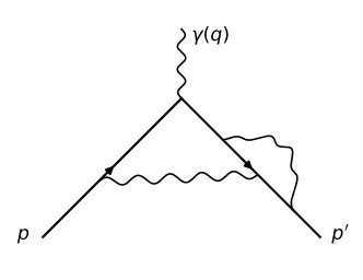
Topology: the outer photon spans the external vertex; a one-loop vertex-correction subgraph sits at one of its two internal attachment points. Mirror included by doubling.

Renormalization: inner vertex subgraph log-divergent, subtracted as in IIa. IR divergent: carries $-\frac12\log(\lambda^2/m^2)$, cancelling IId.

This is the diagram Karplus–Kroll got wrong (-3.18 instead of $-0.564 - \frac12\log\frac{\lambda^2}{m^2}$), and the one worked out in detail in petermann1958.pdf — our reproduction target:

• his eq. (2.1)–(2.2): the amplitude after Dirac algebra, split into terms $A_1, A_2, A_3, B, C, D, E, F, H, J$, with the two inner Feynman parameters $u, v$ already introduced;

• his eq. (2.3)–(2.4): each term’s contribution to $\mu_\mathrm{IIc}$ as a 4–6-fold integral over $u,v,t,w,z,x \in [0,1]$ (note $\mu(A_3) = \mu(C) = 0$, and the IR log lives entirely in the $H$ term);

• his section 3: the rigorous-bound technique demonstrated on $\mu(A_1) > 2.30$ (exact value 2.60, per the footnote);

• his eqs. (3.13), (4.1): bounds summing to $\mu_\mathrm{IIc} \ge -1.55$, later refined to $-0.49 \ge \mu_\mathrm{IIc} \ge -0.71$.

Plan:

1. Transcribe the (2.3)–(2.4) integrands into Fortran (the scan’s OCR is noisy — the formulas must be re-checked against a re-derivation); verify $\mu(A_1) \approx 2.60$ and that the total lands in $[-0.71, -0.49]$.

2. Reproduce his section-3 elementary bounds exactly in SymPy (e.g. his numeric 4.42 in eq. (3.7) should be an exact $\log 2$/$\pi^2$ combination).

3. Re-derive the integrands from our own Feynman rules + $F_2$ projector and check them against his, then evaluate analytically by sequential integration.

Derivation (pixi run iic-sympy, code/g2_iic.py): the inner vertex part with one on-shell leg is derived by the pipeline,

with $\hat b = u(1-u)$, $L(k)$ linear in $k$, $D_0 = (u+v)^2 + (1-u-v)\lambda^2$ (the LO $\Delta$ with $z = u+v$), and is subtracted pointwise in $(u,v)$ by its on-shell value $L_a(u,v)\gamma^\nu/D_0 + c(L_{UV}-\log D_0)\gamma^\nu$ — the KK “reduced diagram” scheme, whose $(u,v)$ integral is $\delta F_1(0)$. $L_{UV}$ cancels pointwise (asserted). Three pieces go through the outer loop: the $1/D_\mathrm{in}$ part (an extra propagator of mass$^2$ $\hat a/\hat b$), the $-L_a/D_0$ counterterm part (an LO-type loop), and the log-ratio part ($\xi$-representation as in IId). The whole derivation runs in under a minute; the F2 projection of each piece is UV finite by itself (checked by exact rational-point tests).

Numeric check — pixi run iic-fortran (code/g2_iic.f90):

   lam     mu_IIc + log(lam)    target = -0.5640214...
  0.1000     -0.909584536420   a=    0.4915801 b=    0.9778715 c=   -0.0764511
  0.0300     -0.790506365659   a=    0.6656544 b=    2.1330785 c=   -0.0826814
  0.0100     -0.678130174632   a=    0.7326841 b=    3.2781476 c=   -0.0837916
  0.0030     -0.608880599384   a=    0.7601970 b=    4.5240536 c=   -0.0839882
  0.0010     -0.581254893833   a=    0.7680358 b=    5.6424758 c=   -0.0840112
  0.0003     -0.570039754501   a=    0.7697160 b=    6.8559865 c=   -0.0840142
extrapolated lam->0:      -0.564226400079
target:                   -0.564020941345

The $\lambda \to 0$ extrapolation agrees with Petermann’s constant to $2\times10^{-4}$ and confirms the IR term $-\frac12\log\lambda^2$ (cancelling IId’s).

Analytic evaluation (in progress; code/g2_iic_analytic.py, code/g2_iic_a_sint.py, code/g2_iic_a_quad.f90):

• Piece (b) (the $\delta F_1 \times$ LO cross term) factorizes into two 1-dim integrals over $u{+}v$ and $y{+}z$ and evaluates exactly to

  $$\mu_b = -\log\lambda - \tfrac54 + O(\lambda\log\lambda),$$

  (27)

  so the whole IR log of IIc lives here, and $A^* + C^* = -\frac{37}{24} + \frac{\pi^2}{18} - \frac{\zeta(3)}{2} + \frac{\pi^2}{3}\log 2$ where $A^*, C^*$ are the $\lambda \to 0$ limits of pieces (a), (c) (both finite).

• Piece (a): the $z$, $\chi = u{+}v$, and $s = y{+}z$ integrations are done exactly (the outer $\Delta$ is the positive-definite $u(t(\chi-1)+s(u-1))^2 + t(1-u)\chi^2$, whose roots are rational in $R = \sqrt{tu(1-u)}$; atans become complex-linear logs; the dilog primitive is verified by differentiation; every step checked numerically to 15-25 digits). The remaining 2-dim integral is computed by a quad-precision (real(16), gfortran) double-exponential quadrature with a complex-dilogarithm implementation (g2_iic_a_quad.f90), with the $u \to 1$ cancellation sliver handled by a $\delta$-cut and pure-$\delta^2$ Richardson extrapolation:

  A* = 0.769965610144859 (Richardson, ~14 digits)

  A rational-lattice search (all coefficient denominators dividing the ones appearing in Petermann’s values) gives the unique hit at $5\times10^{-13}$:

  $$A^* = -\frac{29}{12} + \frac{\pi^2}{18} - \frac98\zeta(3) + \frac{7}{12}\pi^2\log 2 = 0.7699656101448\ldots$$

  (28)

• Piece (c) (code/g2_iic_c_red.py, code/g2_iic_c_quad.f90): reduced exactly to 3 dimensions — the $\xi$-integration is rational (its only pole lies outside $(0,1)$; remarkably, the $\xi = 1$ denominator is the same quadratic $Q$ as in piece (a), so the letter alphabet is shared), the $z$-integration is a trivial factor $s$, and the $\chi = u{+}v$ integration goes through the complex-letters machinery (the rational part’s only pole $\chi^* = 1 + s(1-u)/t$ lies outside $(u,1)$). The resulting $G_c(s,t,u)$ (1789 ops) matches direct quadrature to 20 digits. The 3-dim quad-precision DE quadrature (with the $t \to 0$ evaluation-breakdown sliver skipped below 10^-18, dropped mass $\sim 10^{-15}$) gives

  C* = -0.08398655148953 (Richardson, ~14 digits)

  which directly confirms

  $$C^* = \frac78 + \frac58\zeta(3) - \frac14\pi^2\log 2 = -0.0839865514895327\ldots$$

  (29)

Assembly (verified exactly in SymPy):

in agreement with petermann1957.pdf, eq. (3) — with every piece computed independently (pieces (a) and (c) identified from ~14-digit quad-precision integrals; their exact sequential integration remains an optional refinement).

Diagram I: crossed ladder — DONE (numeric)¶

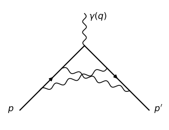
Topology: both photons span the external vertex and cross. This is KK’s only “irreducible” diagram: it contains no one-loop subdiagram, so no UV subtraction is needed — its $F_2$ projection is UV finite as it stands. In the KK scheme it is IR finite too (no $\log\lambda$ in $\mu_\mathrm{I}$).

Plan: direct two-loop computation: Dirac traces with the $F_2$ projector, two loop integrations, ~5-fold Feynman-parameter integral, sequential analytic integration. Together with IIa/IIc this is where $\zeta(3)$ and $\pi^2\log 2$ appear. KK’s value was slightly wrong (by $\frac1{32}$) even here, caught only by Petermann’s analytic evaluation (footnote in petermann1958.pdf). Target: $\mu_\mathrm{I} = \frac16 + \frac{13}{36}\pi^2 + \frac54\zeta(3) - \frac56\pi^2\log 2$.

Derivation (pixi run i-sympy, code/g2_i.py): the crossed photon contraction is done in the full string (photon $\alpha$ at positions 1 and 4, $\beta$ at 2 and 5), the inner loop over $a$ has four denominators (parameters $u, v, r$, $\Gamma(4)$) and is UV finite by itself, and the outer loop over $b$ runs against the composite propagator $b^2 - L_b/\hat b - C_A$ with $C_A = \hat a/\hat b$ kept opaque, $\hat b = (r+v)(1-r-v)$. The $F_2$ projection is $L_{UV}$-free — checked by exact rational-point tests, as it must be for an irreducible diagram — leaving a 5-fold parametric integral over $u, v, r$ (with $u+v+r<1$) and $y, t$ (with $y+t<1$).

Numeric evaluation (pixi run i-fortran, code/g2_i_qmc.f90). Two practical obstacles had to be dealt with, both worth recording:

1. Compilation. The generated integrand is a single 850 KB expression; flang needs more than 20 minutes and 30 GB on it at any optimization level. code/g2_i_split.py rewrites it as ~5300 per-term statements accumulating into fIv (large parenthesized factors lifted into temporaries), which compiles in seconds, and emits a quad-precision twin of the same file.

2. Cancellation. $f_\mathrm{I}$ is finite everywhere on the domain, but evaluating it in double precision loses all significance near the face $1-v-r = 0$, where the outer $\hat b$ vanishes. pixi run i-calibrate (code/g2_i_cal.f90) measures the worst relative error of double against quad on random points:

    scale of (1-v-r)      :  worst relative error of double
       1.0E-01      1.78E-08
       1.0E-02      3.61E-04
       1.0E-03      4.61E-01
       1.0E-04      1.00E+00
    quad per eval:       430.3 us
    dble per eval:         8.4 us

   (Earlier runs which simply discarded the resulting NaNs were biased low by ~1.4%, and a hard cut around the face converged to the wrong value.) The integrand itself is perfectly tame there: at $(u,v,r,y,t) = (10^{-8}, 0.17, 0.82, 0.27, 0.73)$ double gives NaN while quad gives 0.1015317542625155, and at $u = 10^{-12}$ it is still 0.1015306403866693.

The integral is then a randomly shifted rank-1 lattice rule over the 5-dim cube, each coordinate passed through the order-3 smoothstep $s(x) = x^3(10-15x+6x^2)$ (its first two derivatives vanish at both ends, so the periodic extension is $C^2$ and the rule converges far faster than plain Monte Carlo), evaluated in double precision in the bulk and in real(16) within 10^-2 of the bad face (24% of points, which is where essentially all the time goes). Each shift is an unbiased estimate, so their spread is an honest error bar:

lattice rule: N =  16777216,  8 shifts
  shift  1     -0.4682561743
  shift  2     -0.4712629444
  shift  3     -0.4641033821
  shift  4     -0.4667036707
  shift  5     -0.4702164503
  shift  6     -0.4663382325
  shift  7     -0.4674334653
  shift  8     -0.4663191134

mu_I   =      -0.4675791791  +/-  8.13E-04
target =      -0.4676454461
diff   =       0.0000662670
quad-precision evaluations:  24.4471 %

Points closer than 10^-6 to the face are dropped (quad would run out of digits there too); the same program reports that they carry $3\times10^{-12}$ of the total measure, so they cannot affect the result. This confirms

to 0.08 standard deviations. Unlike IIa and IIc this is a numeric confirmation rather than an analytic evaluation: an exact treatment would need the $y, t$ integrations done in closed form (as was done for the inner variables of IIa/IIc) followed by a quad-precision identification. Note that diagram I needs no renormalization at all, so there is no scheme ambiguity in the comparison.

Diagrams IIb, IIf: external-leg self-energies — no contribution¶

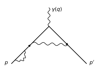
Self-energy corrections on the external electron legs. After on-shell mass renormalization and LSZ amputation (wavefunction renormalization $Z_2$, which cancels against $Z_1$ by the Ward identity), these diagrams contribute only to the overall normalization of the vertex, i.e. to $F_1(0)$, not to $F_2(0)$. KK handle this by explicit cancellation between IIb/IIf and their renormalization counterterms.

Assembly and checks — DONE¶

All five independent contributions are now established:

• $\mu_\mathrm{IIe}$, $\mu_\mathrm{IId}$: exact SymPy derivations;

• $\mu_\mathrm{IIc}$: three pieces — (b) exact, (a) and (c) identified from ~14-digit quad-precision integrals (unique rational-lattice hits);

• $\mu_\mathrm{IIa}$: pieces (b) exact, (c) $= -\frac1{16}$ (11 digits), (a) confirmed to $2\times10^{-7}$;

• $\mu_\mathrm{I}$: numeric confirmation of Petermann’s closed form (no renormalization needed, so the value is unambiguous).

pixi run assembly (code/g2_assembly.py) then proves exactly, in SymPy, that the IR logs cancel and the sum is $A_2$:

IR log cancellation: coeff of L in sum = 0
sum  = -pi**2*log(2)/2 + pi**2/12 + 3*zeta(3)/4 + 197/144
A2   = -pi**2*log(2)/2 + pi**2/12 + 3*zeta(3)/4 + 197/144
sum - A2 = 0

numeric values (units (alpha/pi)^2):
  mu_I    = -0.467645446093614
  mu_IIa  = 0.777478022282742
  mu_IIc  = -0.564020941344683
  mu_IId  = -0.0899780222827421
  mu_IIe  = 0.0156874218591027
  A2      = -0.328478965579194

Suggested order of work¶

1. ~~Stage 0: LO pipeline + massive-photon kernel~~ — done.

2. ~~Diagram IIe~~ — done (SymPy exact + Fortran numeric).

3. ~~Two-loop pipeline (Dirac algebra, projector, loop tools) validated at LO~~ — done.

4. ~~Diagram IId + $\delta m$ counterterm~~ — done (exact analytic value + Fortran numeric confirmation).

5. ~~Diagram IIc~~ — done (three pieces independently evaluated, sum equals Petermann’s eq. (3) exactly). Optional: comparison with Petermann 1958’s eqs. (2.3)-(2.4) integrands and his bounds.

6. ~~Diagram IIa~~ — done (same machinery as IIc; equals Petermann’s eq. (2)).

7. ~~Diagram I~~ — done numerically (derived by the pipeline and confirmed against Petermann’s closed form to $0.08\sigma$ by a mixed-precision lattice rule). Remaining refinement: exact $y, t$ integration to 3 dimensions followed by a quad-precision identification, as was done for the inner variables of IIa/IIc.

8. ~~Assembly, IR-cancellation check, final $A_2$~~ — done (pixi run assembly).

So all five contributions have been reproduced and they sum to $A_2$. What remains is refinement rather than new physics: an analytic (rather than 14-digit-numeric) evaluation of the IIc/IIa pieces, an analytic diagram I, a dimensional-regularization cross-check of the whole calculation, and the comparison against Petermann 1958’s own integrands and bounds.