One diagram in full detail: IId (and IIe as a warm-up)

The two preceding sections attack the order- $\alpha^2$ anomalous moment $A_2$ from two directions. The derivation section goes top-down: it starts from the Green function and stops when each of the five diagrams has been reduced to a well-defined integral. The NLO section goes bottom-up: it takes those integrals, hands them to SymPy and Fortran, and reports numbers. Between the two there is a gap. Nowhere is a single diagram carried continuously, with every intermediate expression written out, from the Lagrangian to a closed-form answer.

That gap is what this section fills, for one diagram. We take IId, the diagram in which a one-loop electron self-energy sits on an internal line of the leading-order vertex, and compute

\mu_\mathrm{IId} = \frac{11}{24} - \frac{\pi^2}{18} + \frac12\log\frac{\lambda^2}{m^2}

(1)

starting from $\mathcal{L}_\mathrm{QED}$ and skipping nothing. IId is the right diagram for this purpose because it needs both kinds of counterterm — a mass counterterm $\delta m$ and a field-strength counterterm $\delta Z_2$ — because its ultraviolet cancellation can be checked by hand in one line, and because it keeps an infrared divergence which we can trace to its source. A shorter warm-up on diagram IIe comes first, to set up the machinery on a diagram that needs only one counterterm.

Everything here is checked by the scripts named along the way, and all displayed outputs are their actual output. Two of the intermediate results are ones SymPy gets wrong if asked naively; both are shown, because knowing where a computer algebra system lies to you is part of knowing how the calculation works.

The reader is assumed to know what a Feynman diagram is and to have seen a one-loop calculation once. No familiarity with renormalization technique is assumed: the counterterms are constructed here, not quoted.

Conventions, fixed once¶

Metric $g_{\mu\nu} = \mathrm{diag}(+1,-1,-1,-1)$ ; Dirac representation for the $\gamma$ matrices, as in code/dirac.py; $\hbar = c = 1$ . The Feynman slash is $\slashed a = \gamma^\mu a_\mu$ , and

\{\gamma^\mu,\gamma^\nu\} = 2g^{\mu\nu},\qquad \sigma^{\mu\nu} = \frac{i}{2}\left[\gamma^\mu,\gamma^\nu\right].

(2)

The electron mass is $m$ ; we set $m=1$ in the parametric integrals (it can always be restored by dimensional analysis) but keep it explicit while deriving. The fine structure constant is $\alpha = e^2/4\pi$ , and the combination that appears in every loop is abbreviated

c \equiv \frac{e^2}{16\pi^2} = \frac{\alpha}{4\pi}.

(3)

Per-diagram results are quoted in units of $(\alpha/\pi)^2$ and written $\mu_\mathrm{X}$ , so that $\sum_\mathrm{X}\mu_\mathrm{X} = A_2$ .

Two regulators are in play throughout:

ultraviolet: Pauli–Villars, which enters through the single symbol $L_{UV} = \log\Lambda^2 + \text{scheme constant}$ . Nothing physical may depend on it, and we will watch it cancel.
infrared: a photon mass $\lambda$ , so the photon propagator is $-ig_{\mu\nu}/(k^2-\lambda^2)$ . Individual diagrams do depend on it; only the sum over diagrams does not.

A word on the photon mass, since a massive vector field is not innocent in general. The propagator of a massive vector is

\frac{-i}{k^2-\lambda^2} \left(g_{\mu\nu} - \frac{k_\mu k_\nu}{\lambda^2}\right),

(4)

and the $k_\mu k_\nu/\lambda^2$ term is singular as $\lambda\to0$ . It is harmless here because the photon always attaches to the electron current, which is conserved: the $k_\mu k_\nu$ piece is contracted with a current $j^\mu$ satisfying $k_\mu j^\mu = 0$ and drops out identically. That is why the 1950s papers could use a photon mass without further apology, and why we may write the propagator simply as $-ig_{\mu\nu}/(k^2-\lambda^2)$ .

1. The Lagrangian and the rules that follow from it¶

1.1 The bare Lagrangian¶

QED with an external classical field $A^\mathrm{cl}_\mu$ is

\mathcal{L} = -\frac14 F_{0\mu\nu}F_0^{\mu\nu} + \bar\psi_0\left(i\slashed\partial - m_0\right)\psi_0 - e_0\bar\psi_0\slashed A_0\psi_0 - e_0\bar\psi_0\slashed A^\mathrm{cl}\psi_0,

(5)

with $F_{0\mu\nu} = \partial_\mu A_{0\nu} - \partial_\nu A_{0\mu}$ . The subscript 0 marks bare quantities: the parameters appearing in the Lagrangian, which are not what an experiment measures. Gauge fixing in Feynman gauge adds $-\frac{1}{2}(\partial^\mu A_{0\mu})^2$ , which is what makes the photon propagator proportional to $g_{\mu\nu}$ .

1.2 Renormalized perturbation theory¶

The reason bare parameters are not the measured ones is that the loop corrections we are about to compute shift them. It is cleaner to say so in the Lagrangian from the start. Define renormalized fields and parameters by

\psi_0 = \sqrt{Z_2}\,\psi,\qquad A_0^\mu = \sqrt{Z_3}\,A^\mu,\qquad m_0 = m + \delta m',\qquad e_0 Z_2\sqrt{Z_3} = e Z_1,

(6)

and write $Z_2 = 1 + \delta_2$ , $Z_3 = 1 + \delta_3$ , $Z_1 = 1 + \delta_1$ . Substituting into $\mathcal{L}$ and separating the terms with a $\delta$ from those without gives

\mathcal{L} = \underbrace{-\frac14 F_{\mu\nu}F^{\mu\nu} + \bar\psi\left(i\slashed\partial - m\right)\psi - e\bar\psi\slashed A\psi - e\bar\psi\slashed A^\mathrm{cl}\psi}_{\text{same form, renormalized parameters}}

(7)

\qquad\underbrace{-\frac14\delta_3F_{\mu\nu}F^{\mu\nu} + \bar\psi\left(i\delta_2\slashed\partial - \delta_m\right)\psi - e\delta_1\bar\psi\slashed A\psi - e\delta_1\bar\psi\slashed A^\mathrm{cl}\psi}_{\text{counterterms}},

(8)

where $\delta_m \equiv Z_2\,\delta m'$ collects the mass shift. The counterterms are ordinary interaction terms with their own Feynman rules; they are not a bookkeeping device applied after the fact. Their values are fixed by renormalization conditions, which is where the physics enters, and we will fix them in §7.

The four counterterms do four different jobs. $\delta_m$ makes the pole of the electron propagator sit at the measured mass $m$ . $\delta_2$ makes the residue at that pole equal to one. $\delta_3$ makes the measured charge the residue of the photon pole. $\delta_1$ renormalizes the vertex, and is tied to $\delta_2$ by the Ward identity $Z_1 = Z_2$ . Diagram IId will need $\delta_m$ and $\delta_2$ ; diagram IIe will need $\delta_3$ .

1.3 The Feynman rules¶

Reading the rules off the Lagrangian in the standard way:

\text{electron propagator:}\qquad \frac{i\left(\slashed k + m\right)}{k^2 - m^2 + i\epsilon}

(9)

\text{photon propagator:}\qquad \frac{-ig_{\mu\nu}}{k^2 - \lambda^2 + i\epsilon}

(10)

\text{vertex:}\qquad -ie\gamma^\mu

(11)

\text{counterterm vertices:}\qquad i\left(\slashed k\,\delta_2 - \delta_m\right),\qquad -ie\,\delta_1\gamma^\mu,

(12)

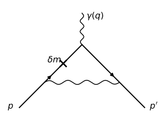
together with the usual $\int d^4k/(2\pi)^4$ per loop, a factor $(-1)$ and a trace for each closed fermion loop, and a relative minus sign between diagrams differing by an interchange of external fermion lines. The two-point counterterm vertex $i(\slashed k\delta_2 - \delta_m)$ is the one that will appear inside IId, drawn as a cross on an electron line.

2. What we are computing¶

2.1 The vertex function and $a_e$ ¶

The object of interest is the amputated three-point function with one photon leg — the vertex function $\Gamma^\mu(p',p)$ , defined so that the scattering amplitude off the external field is

i\mathcal{M} = -ie\,\bar u(p')\,\Gamma^\mu(p',p)\,u(p)\, \tilde A^\mathrm{cl}_\mu(q),\qquad q = p'-p.

(13)

Lorentz invariance, parity and the Ward identity restrict $\Gamma^\mu$ between on-shell spinors to two form factors (this is derived in the LO section):

\bar u(p')\Gamma^\mu u(p) = \bar u(p')\left[\gamma^\mu F_1(q^2) + \frac{i\sigma^{\mu\nu}q_\nu}{2m}F_2(q^2)\right]u(p),

(14)

and the LO section shows that the electron’s magnetic moment is $g/2 = F_1(0) + F_2(0)$ with $F_1(0)=1$ exactly, so that

a_e = \frac{g-2}{2} = F_2(0).

(15)

At order $\alpha$ this is Schwinger’s $\alpha/2\pi$ . We want the order $\alpha^2$ piece, one diagram at a time.

2.2 The Gordon decomposition, derived¶

We will need to convert between the two structures $\gamma^\mu$ and $(p+p')^\mu$ , so let us derive the relation between them explicitly. From $\{\gamma^\mu,\gamma^\nu\} = 2g^{\mu\nu}$ and the definition of $\sigma^{\mu\nu}$ ,

\gamma^\mu\gamma^\nu = \frac12\{\gamma^\mu,\gamma^\nu\} + \frac12\left[\gamma^\mu,\gamma^\nu\right] = g^{\mu\nu} - i\sigma^{\mu\nu}.

(16)

Contract this with $p_\nu$ on the right, and with $p'_\nu$ on the left:

\gamma^\mu\slashed p = p_\nu\gamma^\mu\gamma^\nu = p^\mu - i\sigma^{\mu\nu}p_\nu,

(17)

\slashed p'\gamma^\mu = p'_\nu\gamma^\nu\gamma^\mu = p'^\mu - i\sigma^{\nu\mu}p'_\nu = p'^\mu + i\sigma^{\mu\nu}p'_\nu,

(18)

using the antisymmetry $\sigma^{\nu\mu} = -\sigma^{\mu\nu}$ . Adding,

\gamma^\mu\slashed p + \slashed p'\gamma^\mu = \left(p+p'\right)^\mu + i\sigma^{\mu\nu}\left(p'-p\right)_\nu = \left(p+p'\right)^\mu + i\sigma^{\mu\nu}q_\nu.

(19)

Now sandwich between on-shell spinors and use the Dirac equations $\slashed p\,u(p) = m\,u(p)$ and $\bar u(p')\slashed p' = m\,\bar u(p')$ . The left-hand side becomes $2m\,\bar u(p')\gamma^\mu u(p)$ , so

\bar u(p')\gamma^\mu u(p) = \bar u(p')\left[ \frac{\left(p+p'\right)^\mu}{2m} + \frac{i\sigma^{\mu\nu}q_\nu}{2m}\right]u(p).

(20)

That is the Gordon decomposition. Solving it for $i\sigma^{\mu\nu}q_\nu$ and substituting into the form-factor decomposition gives the form we will actually use,

\Gamma^\mu = \gamma^\mu\left(F_1+F_2\right) - \frac{\left(p+p'\right)^\mu}{2m}F_2 .

(21)

So if we can reduce a computed $\Gamma^\mu$ to the form $\mathcal{A}\gamma^\mu + \mathcal{B}(p+p')^\mu$ , then

F_2 = -2m\,\mathcal{B}.

(22)

One warning about this, which matters later. The two structures $\gamma^\mu$ and $(p+p')^\mu$ are independent as matrices, but not after being sandwiched between spinors at $q=0$ : the Gordon relation at $q = 0$ reads $\bar u\gamma^\mu u = \bar u\,(p+p')^\mu u/2m$ , so the two sandwiches are proportional. Extracting $\mathcal{B}$ therefore requires either keeping $q\ne0$ , or working with the unsandwiched matrix and using the Dirac equation only at the far ends of the string. We do the latter where the algebra is clean, and keep $q\neq0$ where it is not.

2.3 The explicit projector used by the code¶

The scripts do the extraction in a way that is easy to automate: pick the Breit frame, where

p = (E,0,0,w),\qquad p' = (E,0,0,-w),\qquad q = (0,0,0,-2w),

(23)

E = \sqrt{m^2+w^2},\qquad q^2 = -4w^2,

(24)

so both electrons are on shell automatically and $q^2\to0$ means $w\to0$ . Sandwiching with explicit spinors for two choices of $(\mu,s',s)$ gives two independent linear equations for $F_1,F_2$ . Writing $A_\mu^{(s',s)} = \bar u(p',s')\Gamma^\mu u(p,s)$ and using the two choices $(0,\uparrow,\uparrow)$ and $(1,\uparrow,\downarrow)$ , the basis sandwiches evaluate to

\bar u\gamma^0u = 2m,\quad \bar u\frac{i\sigma^{0\nu}q_\nu}{2m}u = -\frac{2w^2}{m} \qquad (\mu=0,\ s'=s=\uparrow),

(25)

\bar u\gamma^1u = -2w,\quad \bar u\frac{i\sigma^{1\nu}q_\nu}{2m}u = -2w \qquad (\mu=1,\ s'=\uparrow,s=\downarrow),

(26)

and solving the $2\times2$ system and letting $w\to0$ gives the shortcut that code/g2_iid.py uses,

F_2(0) = -\frac12\left[A_0\big|_{w=0} + \frac{\partial A_1}{\partial w}\bigg|_{w=0}\right]\qquad (m=1).

(27)

Note that the $\mu=1$ sandwich alone would be degenerate — it measures only the combination $F_1+F_2$ , since both basis structures equal $-2w$ — which is the same degeneracy noted above, and the reason a second sandwich is needed.

3. From the Green function to this diagram¶

3.1 Gell-Mann–Low and Dyson¶

Everything starts from the time-ordered Green function of interacting fields,

G^\mu(x';y;x) = \langle\Omega|T\,\psi(x')A^\mu(y)\bar\psi(x)|\Omega\rangle,

(28)

which the Gell-Mann–Low theorem rewrites in terms of free fields and the interaction Hamiltonian,

G^\mu = \frac{\langle0|T\,\psi_I(x')A_I^\mu(y)\bar\psi_I(x)\, \exp\left(i\int d^4z\,\mathcal{L}_\mathrm{int}\right)|0\rangle} {\langle0|T\exp\left(i\int d^4z\,\mathcal{L}_\mathrm{int}\right)|0\rangle}.

(29)

Expanding the exponential is the Dyson series. With $\mathcal{L}_\mathrm{int} = -e\bar\psi\slashed A\psi$ the term with $n$ interaction vertices is

\frac{(-ie)^n}{n!}\int d^4z_1\cdots d^4z_n\; \langle0|T\,\psi(x')A^\mu(y)\bar\psi(x)\, \left(\bar\psi\slashed A\psi\right)(z_1)\cdots \left(\bar\psi\slashed A\psi\right)(z_n)|0\rangle,

(30)

and the denominator cancels exactly the disconnected vacuum pieces of the numerator.

3.2 Which order do we need?¶

Count powers of $e$ . The external-field vertex carries one power; each internal photon carries two (one at each end). The leading-order vertex correction has one internal photon: $e^1\cdot e^2 = e^3$ . The two-loop corrections have two internal photons: $e^1\cdot e^4 = e^5$ . Since $a_e$ is measured in units where the LO term is $\alpha/2\pi \propto e^2$ relative to the tree vertex, the order $e^5$ terms give the $(\alpha/\pi)^2$ contributions. So we want $n=5$ .

In addition there are terms with counterterm vertices. A counterterm is itself of order $e^2$ (it is fixed by a one-loop calculation), so a diagram with three ordinary vertices and one two-point counterterm is also of order $e^3\cdot e^2 = e^5$ and must be included. That is exactly the $\delta m$ insertion diagram which pairs with IId.

3.3 Wick’s theorem and the contraction that gives IId¶

Wick’s theorem turns the vacuum expectation value into a sum over complete pairings of the fields, each pairing contributing a product of propagators, with a sign $(-1)^P$ for the permutation $P$ needed to bring the paired fermion operators adjacent. For our correlator at order $n=5$ there are $6!$ ways to pair the six $\psi$ ’s with the six $\bar\psi$ ’s and 15 ways to pair the six photon fields (three from the $z_i$ vertices plus the external one — more precisely, at order 5 there are five vertex photons and one external, giving $(6-1)!! = 15$ perfect matchings), for a total of $15\times 6! = 10800$ complete contractions.

code/wick_enum.py enumerates all of them and classifies each by topology and fermion-loop count. The relevant rows of its output are

order e^5:  10800 complete contractions (15 photon matchings x 6! fermion pairings)
  topology class                                                      count  /n! sign
  IIc: corner, vertex part at an internal vertex (+ mirror)             240    2 +1
  IId: self-energy on an internal line (+ mirror)                       240    2 +1
  I: crossed ladder                                                     120    1 +1
  IIa: ladder (vertex part at the external vertex)                      120    1 +1
  IIe: vacuum polarization in the internal photon                       120    1 -1

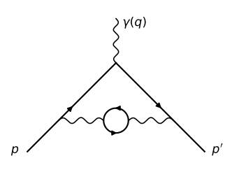
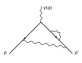
Read the IId row: 240 contractions, which after dividing by the $5!$ from the Dyson denominator gives weight 2. That factor of two is not a symmetry factor; it is the statement that there are two distinct diagrams of this topology — the self-energy can sit on either of the two internal electron lines — and they are mirror images of one another. The Breit-frame projection is symmetric under the reflection that exchanges them, so we compute one and double it. The sign is +1: IId has no closed fermion loop. (IIe’s -1 in the last row is the closed-loop sign, and it is already included in the standard definition of $\Pi^{\mu\nu}$ .)

Concretely, one of the 240 contractions is the following. Label the five vertices $z_1,\dots,z_5$ in the order in which the fermion line visits them, running from the incoming electron at $x$ to the outgoing one at $x'$ . Let the external photon attach at $z_4$ . Contract the photon field at $z_1$ with the one at $z_5$ : that is the outer photon, and since $z_4$ lies between them it spans the external vertex, which is the leading-order vertex topology. Contract the remaining two photon fields, at $z_2$ and $z_3$ , with each other: these are adjacent vertices with no external attachment between them, so the blob they form is a self-energy correction sitting on the internal electron line that runs from $z_1$ to $z_4$ .

That distinction is the whole taxonomy in one sentence. If the inner photon had spanned the external vertex ( $z_2$ to $z_5$ , say) we would have a vertex subgraph and the diagram would be IIc or IIa; because it connects two adjacent vertices on a single internal segment, it is a self-energy and the diagram is IId. All 240 members of the class differ from this one by relabelling the $z_i$ , which the $1/5!$ absorbs, and by the mirror reflection that puts the blob on the $z_4$ – $z_5$ segment instead.

3.4 What LSZ does with the rest¶

Most of the 10800 contractions never reach $\Gamma^\mu$ :

External-leg corrections (840 + 240 + ... contractions) are self-energy blobs on the incoming or outgoing electron line. LSZ amputates the external propagators and supplies one factor of $\sqrt{Z_2}$ per external fermion leg; the effect of all these diagrams is precisely to build the full propagator whose residue $Z_2$ is then divided out. They contribute nothing to compute.
External-potential corrections (classes III and IV) dress the photon line carrying $q$ . After the charge renormalization of §1.2 they contribute $\hat\Pi(0)=0$ at $q^2\to0$ .
Odd fermion loops (class V) cancel in pairs by Furry’s theorem.
Disconnected and tadpole pieces cancel against the denominator or vanish by symmetric integration.

What remains is the five 1PI vertex cores, of which IId is one.

4. Where the Feynman rules come from: one contraction, done by hand¶

Section 1.3 listed the Feynman rules and §3 said which contraction we want, but between those two statements there is a real calculation: Wick’s theorem produces a sum of position-space products of propagators, and turning one of those products into a momentum-space integral is what defines the rules. This section does that calculation once, completely, on the simplest nontrivial case — the one-loop vertex correction at order $e^3$ — and then adds the one rule that cannot be seen at that order, the closed fermion loop, which is exactly the ingredient diagram IIe needs.

Nothing here is quoted. We start from the Dyson series and end with

\bar u(p')\,\delta\Gamma^\mu_\mathrm{LO}\,u(p) = \int\frac{\mathrm{d}^4k}{(2\pi)^4}\; \bar u(p')\,(-ie\gamma^\nu)\, \frac{i(\slashed{k}'+m)}{k'^2-m^2}\,\gamma^\mu\, \frac{i(\slashed{k}+m)}{k^2-m^2}\,(-ie\gamma^\rho)\,u(p)\; \frac{-ig_{\nu\rho}}{k_\gamma^2-\lambda^2},

(31)

which is the formula §6.1 takes as its starting point. Once it has been obtained this way, the “rules” are visible as a pattern in the answer, and no further contraction ever has to be done by hand.

4.1 The two propagators¶

Wick’s theorem expresses a time-ordered vacuum expectation value as a sum over complete pairings, each pairing contributing a product of contractions, and a contraction of two free fields is by definition the free two-point function. For the two fields we have:

\overline{\psi_a(x)\,\bar\psi_b(y)} \equiv \langle0|T\,\psi_a(x)\bar\psi_b(y)|0\rangle = S_{ab}(x-y),

(32)

\overline{A_\alpha(x)\,A_\beta(y)} \equiv \langle0|T\,A_\alpha(x)A_\beta(y)|0\rangle = D_{\alpha\beta}(x-y).

(33)

Both are Green functions of the corresponding free wave operator, which fixes them without any further work. The Dirac field satisfies $(i\slashed\partial - m)\psi = 0$ , and the time-ordering step function produces a contact term, giving

\left(i\slashed\partial_x - m\right)S(x-y) = i\,\delta^4(x-y).

(34)

Writing $S(x-y) = \int\frac{d^4k}{(2\pi)^4}e^{-ik\cdot(x-y)}\tilde S(k)$ and using $i\slashed\partial_x e^{-ikx} = \slashed k\,e^{-ikx}$ ,

\left(\slashed k - m\right)\tilde S(k) = i \quad\Longrightarrow\quad \tilde S(k) = \frac{i}{\slashed k - m} = \frac{i\left(\slashed k+m\right)}{k^2-m^2},

(35)

where the last step multiplies numerator and denominator by $\slashed k+m$ and uses $\slashed k\slashed k = k^2$ . The $+i\epsilon$ that selects the Feynman contour is understood. The same argument for the photon in Feynman gauge, where the wave operator is $-g_{\alpha\beta}\,\partial^2$ (plus the mass term $\lambda^2$ ), gives

\tilde D_{\alpha\beta}(k) = \frac{-ig_{\alpha\beta}}{k^2-\lambda^2}.

(36)

These two expressions are the entire input. Everything else below is combinatorics and Fourier transforms.

4.2 The Dyson series at order $e^3$ , written out¶

From §3.1, the term of the Green function with three interaction vertices is

G^{\mu,(3)}(x',y,x) = \frac{i^3}{3!}\int d^4z_1\,d^4z_2\,d^4z_3\; \langle0|T\,\psi(x')A^\mu(y)\bar\psi(x)\, \mathcal{L}_\mathrm{int}(z_1)\mathcal{L}_\mathrm{int}(z_2) \mathcal{L}_\mathrm{int}(z_3)|0\rangle,

(37)

and with $\mathcal{L}_\mathrm{int}(z) = -e\,\bar\psi(z)\gamma^\alpha\psi(z)A_\alpha(z)$ each factor $i\mathcal{L}_\mathrm{int}$ carries $i\cdot(-e) = -ie$ :

G^{\mu,(3)} = \frac{\left(-ie\right)^3}{3!} \int d^4z_1\,d^4z_2\,d^4z_3\; \langle0|T\,\psi(x')A^\mu(y)\bar\psi(x)\, \left(\bar\psi\gamma^{\alpha_1}\psi A_{\alpha_1}\right)(z_1) \left(\bar\psi\gamma^{\alpha_2}\psi A_{\alpha_2}\right)(z_2) \left(\bar\psi\gamma^{\alpha_3}\psi A_{\alpha_3}\right)(z_3)|0\rangle.

(38)

There is the first Feynman rule already: the factor $-ie$ per vertex is nothing but $i$ from the Dyson exponential times the coupling $-e$ from the Lagrangian. The $\gamma^{\alpha_i}$ that accompanies it is the Dirac structure of the interaction term.

4.3 Counting the contractions¶

The fields to be paired are, on the fermion side,

\psi(x'),\ \psi(z_1),\ \psi(z_2),\ \psi(z_3) \qquad\text{and}\qquad \bar\psi(x),\ \bar\psi(z_1),\ \bar\psi(z_2),\ \bar\psi(z_3),

(39)

four of each, hence $4! = 24$ ways to pair them; and on the photon side

A^\mu(y),\ A_{\alpha_1}(z_1),\ A_{\alpha_2}(z_2),\ A_{\alpha_3}(z_3),

(40)

four fields, hence 3 perfect matchings (4 objects pair up in $3!! = 3$ ways). In total $24\times3 = 72$ complete contractions, which is exactly what code/wick_enum.py reports:

order e^3:  72 complete contractions (3 photon matchings x 4! fermion pairings)

Its classification of those 72 is

topology class                                                      count  /n! sign
  tadpole loop  tr[gamma S(0)] = 0                                       39    - +1/-1
  external-leg corrections only (tree vertex)                            12    2 +1
  III: VP on the external-potential line x tree vertex                    6    1 -1
  LO one-loop vertex correction                                           6    1 +1
  forward line x (rest): no scattering / disconnected                     6    1 -1
  disconnected (vacuum bubble or detached blob)                           3    - -1
  total                                                                  72   12

and we now take the fourth row apart.

4.4 The contraction we want¶

Choose the pairing in which the fermion line runs $x\to z_1\to z_2\to z_3\to x'$ , the external photon at $y$ attaches to the middle vertex $z_2$ , and the photons at $z_1$ and $z_3$ contract with each other:

\overline{\psi(x')\bar\psi(z_3)},\quad \overline{\psi(z_3)\bar\psi(z_2)},\quad \overline{\psi(z_2)\bar\psi(z_1)},\quad \overline{\psi(z_1)\bar\psi(x)},

(41)

\overline{A^\mu(y)A_{\alpha_2}(z_2)},\qquad \overline{A_{\alpha_1}(z_1)A_{\alpha_3}(z_3)}.

(42)

Because the internal photon connects $z_1$ and $z_3$ while the external photon sits at $z_2$ between them, this photon spans the external vertex: it is the one-loop vertex correction.

4.5 The Dirac indices chain into a matrix product¶

Write the vertex bilinears with explicit spinor indices, so that everything is a product of anticommuting numbers with $c$ -number $\gamma$ ’s in between:

\left(\bar\psi\gamma^{\alpha}\psi\right)(z) = \bar\psi_i(z)\left(\gamma^{\alpha}\right)_{ij}\psi_j(z).

(43)

Each bilinear contains two fermion fields, so it is Grassmann-even and commutes with everything: we may reorder the three vertex factors at will, without any sign. Choose the order $z_3,z_2,z_1$ and write the whole fermion string as

\psi_a(x')\; \left[\bar\psi_{i_3}(z_3)\gamma^{\alpha_3}_{i_3j_3}\psi_{j_3}(z_3)\right] \left[\bar\psi_{i_2}(z_2)\gamma^{\alpha_2}_{i_2j_2}\psi_{j_2}(z_2)\right] \left[\bar\psi_{i_1}(z_1)\gamma^{\alpha_1}_{i_1j_1}\psi_{j_1}(z_1)\right] \bar\psi_b(x).

(44)

Now read the fields left to right:

\psi_a(x'),\ \bar\psi_{i_3}(z_3),\ \psi_{j_3}(z_3),\ \bar\psi_{i_2}(z_2),\ \psi_{j_2}(z_2),\ \bar\psi_{i_1}(z_1),\ \psi_{j_1}(z_1),\ \bar\psi_b(x).

(45)

Every contraction we want is between neighbours: the 1st with the 2nd, the 3rd with the 4th, the 5th with the 6th, the 7th with the 8th. No field has to be moved past any other, so

\boxed{\ \text{the fermion sign of an open line is } +1.\ }

(46)

This is not an accident of this diagram. Any open fermion line can be brought to this form by reordering the (even) bilinears along the line, so every diagram without a closed loop has sign +1; the signs that matter are the relative ones between diagrams that exchange external legs, and the $(-1)$ per closed loop derived in §4.10.

The spinor indices now chain automatically:

S_{a i_3}(x'-z_3)\,\gamma^{\alpha_3}_{i_3 j_3}\, S_{j_3 i_2}(z_3-z_2)\,\gamma^{\alpha_2}_{i_2 j_2}\, S_{j_2 i_1}(z_2-z_1)\,\gamma^{\alpha_1}_{i_1 j_1}\, S_{j_1 b}(z_1-x),

(47)

each repeated index summed with its neighbour. This is a matrix product, read from the outgoing end to the incoming end — which is why Feynman diagrams are written right-to-left along the fermion line. That convention is a consequence of the index bookkeeping, not a choice.

Including the photon contractions, the contribution of this one pairing to $G^{\mu,(3)}$ is

\frac{\left(-ie\right)^3}{3!}\int d^4z_1d^4z_2d^4z_3\; \left[S(x'-z_3)\gamma^{\alpha_3}S(z_3-z_2)\gamma^{\alpha_2} S(z_2-z_1)\gamma^{\alpha_1}S(z_1-x)\right]

(48)

\times\;D^{\mu}{}_{\alpha_2}(y-z_2)\; D_{\alpha_1\alpha_3}(z_1-z_3).

(49)

4.6 Why the $1/3!$ disappears¶

The pairing above is one of the 72. But five others give exactly the same expression: the three labels $z_1,z_2,z_3$ can be assigned to the three roles (first vertex on the line, external-photon vertex, last vertex) in $3! = 6$ ways, and since $z_1,z_2,z_3$ are integration variables, relabelling them turns any one of those six into any other. They are six distinct terms of Wick’s theorem with identical values.

That is the count wick_enum.py reports for this class, and it cancels the Dyson denominator exactly:

\frac{1}{3!}\times 6 = 1 .

(50)

The same argument works at every order — the $n!$ ways of relabelling $n$ vertices cancel the $1/n!$ — which is why the rules carry no factorials. (The classes whose count is not $n!$ are the ones with a genuine symmetry factor; wick_enum.py’s “/n!” column is exactly this weight, and it is 1 here.) So

G^{\mu,(3)}_\mathrm{vertex} = \left(-ie\right)^3 \int d^4z_1d^4z_2d^4z_3\; \left[S\gamma S\gamma S\gamma S\right]\,D\,D

(51)

with the arguments as above.

4.7 To momentum space¶

Substitute the Fourier representation of every propagator. Give each one a momentum flowing in the direction of its first argument minus its second, i.e. write $S(a-b) = \int_k e^{-ik\cdot(a-b)}\tilde S(k)$ with $\int_k \equiv \int d^4k/(2\pi)^4$ , so that $k$ flows from $b$ to $a$ . Name the momenta

k_0:\ x\to z_1,\qquad k:\ z_1\to z_2,\qquad k':\ z_2\to z_3,\qquad k_4:\ z_3\to x',

(52)

\ell:\ z_1\to z_3\ \text{(internal photon)},\qquad q:\ y\to z_2\ \text{(external photon)},

(53)

which means writing the two photon contractions as $D_{\alpha_3\alpha_1}(z_3-z_1)$ and $D_{\alpha_2}{}^{\mu}(z_2-y)$ — both allowed, since $D_{\alpha\beta}(a-b) = D_{\beta\alpha}(b-a)$ because the photon propagator is even in its momentum.

Now every $z_i$ appears only in exponentials, and each $z$ integral is a delta function. Collect the phases at $z_1$ : the propagator $S(z_1-x)$ contributes $e^{-ik_0z_1}$ , the propagator $S(z_2-z_1)$ contributes $e^{+ikz_1}$ , and $D(z_3-z_1)$ contributes $e^{+i\ell z_1}$ , so

\int d^4z_1\;e^{i\left(k+\ell-k_0\right)z_1} = \left(2\pi\right)^4\delta^4\left(k+\ell-k_0\right) \quad\Longrightarrow\quad k_0 = k+\ell .

(54)

Likewise at $z_2$ (phases $e^{-ikz_2}$ , $e^{+ik'z_2}$ , $e^{-iqz_2}$ ) and at $z_3$ (phases $e^{-ik'z_3}$ , $e^{+ik_4z_3}$ , $e^{-i\ell z_3}$ ):

\int d^4z_2 \;\Rightarrow\; k' = k+q, \qquad \int d^4z_3 \;\Rightarrow\; k_4 = k'+\ell .

(55)

This is the rule “momentum is conserved at every vertex”, and it comes from nothing but the $z$ integration of plane waves. Three delta functions against four propagator momenta plus the external ones leave exactly one momentum unfixed — the loop momentum — with its $\int d^4k/(2\pi)^4$ left over. That is the rule “one unconstrained integration per loop.”

4.8 Amputation, and the answer¶

The external legs carry $k_0$ and $k_4$ and the external photon carries $q$ . LSZ instructs us to Fourier transform in $x,x',y$ , put the external momenta on shell, strip the three external propagators, and replace the external fermion legs by the spinors $u(p)$ and $\bar u(p')$ . So we set

k_0 = p,\qquad k_4 = p',

(56)

and drop $\tilde S(p)$ , $\tilde S(p')$ and the external photon propagator, leaving its index $\mu$ at the vertex $z_2$ . From $k_0 = k+\ell$ ,

\ell = p - k,

(57)

so the internal photon carries $p-k$ ; since it enters only through $\ell^2 = (p-k)^2 = (k-p)^2$ , this is the $k_\gamma = k-p$ of §6.1. And from $k' = k+q$ the second fermion propagator carries $k+q$ , as advertised. The one remaining integration is over $k$ .

Finally, $\Gamma^\mu$ was defined in §2.1 with the external-vertex factor $-ie$ stripped off, so the vertex at $z_2$ contributes a bare $\gamma^\mu$ and only two factors of $-ie$ survive. Putting it together, and renaming $\alpha_3\to\nu$ , $\alpha_1\to\rho$ :

\boxed{\;\bar u(p')\,\delta\Gamma^\mu_\mathrm{LO}\,u(p) = \int\frac{\mathrm{d}^4k}{(2\pi)^4}\; \bar u(p')\,(-ie\gamma^\nu)\, \frac{i(\slashed{k}'+m)}{k'^2-m^2}\,\gamma^\mu\, \frac{i(\slashed{k}+m)}{k^2-m^2}\,(-ie\gamma^\rho)\,u(p)\; \frac{-ig_{\nu\rho}}{k_\gamma^2-\lambda^2}\;}

(58)

which is precisely the expression §6.1 starts from — now derived rather than quoted.

4.9 Reading off the rules¶

Look at what the derivation produced, and where each piece came from:

in the answer	came from
$-ie\gamma^\alpha$ per vertex	$i$ from the Dyson exponential $\times$ $-e\gamma^\alpha$ from $\mathcal{L}_\mathrm{int}$ (§4.2)
$i(\slashed k+m)/(k^2-m^2)$ per internal fermion line	the contraction $\tilde S(k)$ , i.e. the Dirac Green function (§4.1)
$-ig_{\alpha\beta}/(k^2-\lambda^2)$ per internal photon line	the contraction $\tilde D(k)$ (§4.1)
matrices multiplied against the fermion arrow	the chaining of spinor indices (§4.5)
no $1/n!$	cancelled by the $n!$ vertex relabellings (§4.6)
momentum conserved at each vertex	the $\int d^4z$ of plane waves (§4.7)
$\int d^4k/(2\pi)^4$ per loop	the momentum left unfixed by those deltas (§4.7)
$\bar u(p')\ldots u(p)$ , no external propagators	LSZ amputation (§4.8)
overall sign +1	open fermion line, all contractions adjacent (§4.5)

That table is §1.3. From here on we use it as a shortcut, having seen that it is a shortcut and not an axiom.

4.10 The rule that needs order $e^5$ : closed fermion loops¶

One rule cannot be seen at order $e^3$ in a vertex diagram, and it is the one diagram IIe depends on. Consider a contraction in which two vertices $z_a$ and $z_b$ have their fermion fields paired with each other in both directions,

\overline{\psi(z_a)\bar\psi(z_b)}\quad\text{and}\quad \overline{\psi(z_b)\bar\psi(z_a)},

(59)

so that the fermion line closes on itself. Write the two bilinears with indices, in the order they appear:

\left[\bar\psi_i(z_a)\Gamma^{(a)}_{ij}\psi_j(z_a)\right] \left[\bar\psi_k(z_b)\Gamma^{(b)}_{kl}\psi_l(z_b)\right],

(60)

so the fields in order are $\bar\psi_i(z_a),\ \psi_j(z_a),\ \bar\psi_k(z_b),\ \psi_l(z_b)$ .

The first contraction, $\psi_j(z_a)$ with $\bar\psi_k(z_b)$ , is between neighbours (positions 2 and 3): no sign, and it gives $S_{jk}(z_a-z_b)$ .

The second is the problem. What is left is $\bar\psi_i(z_a)\,\psi_l(z_b)$ — in that order — whereas the contraction is defined as $\langle0|T\,\psi_l(z_b)\bar\psi_i(z_a)|0\rangle = S_{li}(z_b-z_a)$ , with $\psi$ to the left of $\bar\psi$ . Since these are anticommuting fields, exchanging them costs a minus sign:

\bar\psi_i(z_a)\,\psi_l(z_b) = -\,\psi_l(z_b)\,\bar\psi_i(z_a) \quad\Longrightarrow\quad \overline{\bar\psi_i(z_a)\,\psi_l(z_b)} = -\,S_{li}(z_b-z_a).

(61)

One transposition, one minus sign. Collecting the two contractions with the $\gamma$ ’s:

-\,\Gamma^{(a)}_{ij}\,S_{jk}(z_a-z_b)\,\Gamma^{(b)}_{kl}\, S_{li}(z_b-z_a),

(62)

and now note the index pattern: $i$ starts the chain and $i$ also ends it. The chain closes, and a matrix product whose first and last index are summed together is a trace:

\boxed{\;= -\,\mathrm{tr}\left[\Gamma^{(a)}\,S(z_a-z_b)\, \Gamma^{(b)}\,S(z_b-z_a)\right].\;}

(63)

Both special features of a closed fermion loop — the overall $(-1)$ and the Dirac trace — come from this single reordering. The minus sign is the anticommutativity of the fields; the trace is the fact that a closed line has no free spinor index. The argument generalizes to a loop with any number $n$ of vertices: $n-1$ of the contractions are between neighbours and the last one closes the cycle at the cost of one transposition, so the sign is $(-1)$ per loop regardless of its size.

Applying this to two vertices joined to the rest of the diagram by photons of indices $\mu,\nu$ , going to momentum space exactly as in §4.7, and calling the loop momentum $l$ and the photon momentum $k$ :

i\Pi^{\mu\nu}(k) = \left(-1\right)\int\frac{\mathrm{d}^4l}{(2\pi)^4}\; \mathrm{tr}\left[\left(-ie\gamma^\mu\right) \frac{i\left(\slashed l+m\right)}{l^2-m^2} \left(-ie\gamma^\nu\right) \frac{i\left(\slashed l-\slashed k+m\right)} {\left(l-k\right)^2-m^2}\right],

(64)

which is the definition §6.1 uses. Its two internal fermion lines are the two contractions above; its $(-1)$ and its trace are what we just derived; and its $(-ie\gamma)$ 's, its propagators and its single loop integration are the rules of §4.9.

Diagram IIe is then the contraction, at order $e^5$ , in which the internal photon of §4.4 is cut and this loop inserted between the two halves — which in momentum space is exactly the replacement

\frac{-ig_{\nu\rho}}{k_\gamma^2-\lambda^2}\;\longrightarrow\; \frac{-ig_{\nu\alpha}}{k_\gamma^2-\lambda^2}\; \left[i\Pi^{\alpha\beta}(k_\gamma)\right]\; \frac{-ig_{\beta\rho}}{k_\gamma^2-\lambda^2}

(65)

that §6.1 performs. Nothing else about IIe requires a new rule.

4.11 The counterterm vertices¶

The counterterm terms of §1.2 are ordinary interaction terms, so they go through the identical derivation. From

\mathcal{L}_\mathrm{ct} \supset \bar\psi\left(i\delta_2\slashed\partial - \delta_m\right)\psi,

(66)

the same $i$ from the Dyson exponential and the same Fourier transform $i\slashed\partial\to\slashed k$ give a two-point vertex

i\left(\slashed k\,\delta_2 - \delta_m\right),

(67)

which is the rule quoted in §1.3 and the one that will be inserted on an electron line in §9.1. Its value is not fixed by this construction — it is fixed by the renormalization conditions of §8.2, which is the whole content of renormalization.

5. The loop-integration toolkit¶

Both diagrams below arrive in the same shape: a polynomial numerator divided by a product of propagator denominators,

\int\frac{\mathrm{d}^4k}{(2\pi)^4}\; \frac{N(k)}{P_1(k)^{n_1}\,P_2(k)^{n_2}\cdots P_j(k)^{n_j}}, \qquad P_i(k) = \left(k-a_i\right)^2 - m_i^2 + i\epsilon,

(68)

where $N$ is a polynomial in the components $k^\mu$ (produced by the $\slashed{k}$ 's of the fermion propagators and the $\gamma$ ’s of the vertices), each $a_i$ is a fixed combination of external momenta, and $m_i$ is $m$ for an electron line and $\lambda$ for a photon line. Nothing in this section depends on which diagram produced the expression.

There are five mechanical steps: merge the denominators into a single quadratic in $k$ (§5.1), complete the square and shift (§5.2), rotate the contour to Euclidean space (§5.3), do the radial integral (§5.4, with the divergent case in §5.5), and use rotational invariance to strip the loop momentum out of the numerator (§5.6). They are exactly the contents of code/loops.py, and each formula below is quoted together with the function that implements it. §5.7 collects the $\gamma$ -matrix contraction identities that make the numerator algebra short by hand, and §5.8 sets up just enough dimensional regularization to redo the one divergent case independently.

5.1 Feynman parameters¶

Two denominators. Let $A$ and $B$ be two nonzero complex numbers such that the straight segment joining them does not pass through the origin. (This is guaranteed by the $i\epsilon$ : every $P_i$ carries the same sign of the infinitesimal imaginary part, so any convex combination $uA+(1-u)B$ has that sign too and cannot vanish.) Then the function

u \;\longmapsto\; \frac{-1}{(A-B)\left[B+u(A-B)\right]}

(69)

is well defined for $u\in[0,1]$ , and differentiating it gives

\frac{\mathrm{d}}{\mathrm{d}u} \left[\frac{-1}{(A-B)\left[B+u(A-B)\right]}\right] = \frac{-1}{(A-B)}\cdot\frac{-(A-B)}{\left[B+u(A-B)\right]^2} = \frac{1}{\left[B+u(A-B)\right]^2}.

(70)

Since $B+u(A-B) = uA+(1-u)B$ , the fundamental theorem of calculus gives

\int_0^1\frac{\mathrm{d}u}{\left[uA+(1-u)B\right]^2} = \left[\frac{-1}{(A-B)\left(B+u(A-B)\right)}\right]_{u=0}^{u=1} = \frac{-1}{A-B}\left(\frac{1}{A}-\frac{1}{B}\right),

(71)

and, using $\frac1A-\frac1B = \frac{B-A}{AB}$ ,

\int_0^1\frac{\mathrm{d}u}{\left[uA+(1-u)B\right]^2} = \frac{-1}{A-B}\cdot\frac{B-A}{AB} = \frac{1}{AB}.

(72)

This is the base case. Note that it is already of the general form: with $u_1 = u$ and $u_2 = 1-u$ the integral reads

\frac{1}{AB} = \int_0^1\mathrm{d}u_1\,\mathrm{d}u_2\; \delta\!\left(1-u_1-u_2\right) \frac{1}{\left[u_1A+u_2B\right]^{2}} .

(73)

Repeated denominators. Both sides of the base case are functions of $A$ and $B$ , so we may differentiate. From $\partial_A^{\,p}A^{-1} = (-1)^p\,p!\,A^{-1-p}$ ,

\partial_A^{\,n_1-1}\partial_B^{\,n_2-1}\frac{1}{AB} = (-1)^{n_1-1}(n_1-1)!\,(-1)^{n_2-1}(n_2-1)!\; \frac{1}{A^{n_1}B^{n_2}}.

(74)

On the other side, differentiating under the integral sign and using $\partial_A\left[uA+(1-u)B\right] = u$ , $\partial_B\left[uA+(1-u)B\right] = 1-u$ ,

\partial_A^{\,p}\,\frac{1}{\left[uA+(1-u)B\right]^{2}} = (-1)^p\,2\cdot3\cdots(p+1)\; \frac{u^{p}}{\left[uA+(1-u)B\right]^{2+p}} = \frac{(-1)^p(p+1)!\;u^{p}}{\left[uA+(1-u)B\right]^{2+p}},

(75)

and applying $\partial_B^{\,q}$ to that result in the same way,

\partial_A^{\,p}\partial_B^{\,q}\, \frac{1}{\left[uA+(1-u)B\right]^{2}} = \frac{(-1)^{p+q}(p+q+1)!\;u^{p}(1-u)^{q}} {\left[uA+(1-u)B\right]^{2+p+q}}.

(76)

Setting $p = n_1-1$ , $q = n_2-1$ (so $p+q+1 = n_1+n_2-1$ and $2+p+q = n_1+n_2$ ), the common sign $(-1)^{n_1+n_2-2}$ cancels between the two sides and we are left with

\frac{1}{A^{n_1}B^{n_2}} = \frac{(n_1+n_2-1)!}{(n_1-1)!\,(n_2-1)!} \int_0^1\mathrm{d}u\; \frac{u^{n_1-1}(1-u)^{n_2-1}}{\left[uA+(1-u)B\right]^{n_1+n_2}} = \frac{\Gamma(n_1+n_2)}{\Gamma(n_1)\Gamma(n_2)} \int_0^1\mathrm{d}u\; \frac{u^{n_1-1}(1-u)^{n_2-1}}{\left[uA+(1-u)B\right]^{n_1+n_2}}.

(77)

Induction to $k$ denominators. Write $N \equiv \sum_{i=1}^{k}n_i$ and $N' \equiv \sum_{i=1}^{k-1}n_i$ , and assume the claimed formula for $k-1$ denominators,

\frac{1}{A_1^{n_1}\cdots A_{k-1}^{n_{k-1}}} = \frac{\Gamma(N')}{\prod_{i<k}\Gamma(n_i)} \int_0^1\prod_{i<k}\mathrm{d}u_i\; \delta\!\left(1-\sum_{i<k}u_i\right) \frac{\prod_{i<k}u_i^{\,n_i-1}} {\left[\sum_{i<k}u_iA_i\right]^{N'}} .

(78)

Multiply by $A_k^{-n_k}$ and apply the two-denominator formula to the pair $\left(\sum_{i<k}u_iA_i\right)^{N'}$ and $A_k^{n_k}$ , calling the new parameter $v$ :

\frac{1}{\prod_{i\le k}A_i^{n_i}} = \frac{\Gamma(N)}{\prod_{i\le k}\Gamma(n_i)} \int_0^1\mathrm{d}v\;v^{N'-1}(1-v)^{n_k-1} \int_0^1\prod_{i<k}\mathrm{d}u_i\; \delta\!\left(1-\sum_{i<k}u_i\right) \frac{\prod_{i<k}u_i^{\,n_i-1}} {\left[v\sum_{i<k}u_iA_i+(1-v)A_k\right]^{N}} ,

(79)

where the two $\Gamma(N')$ factors cancelled. It remains to show that this double integral is the symmetric $k$ -parameter expression. Change variables from $(u_1,\dots,u_{k-1},v)$ to $(x_1,\dots,x_k)$ by

x_i = v\,u_i\quad(i<k), \qquad x_k = 1-v ,

(80)

which is one-to-one from the region $\{u_i\ge0,\ \sum_{i<k}u_i=1,\ 0\le v\le1\}$ onto $\{x_i\ge0,\ \sum_{i\le k}x_i=1\}$ , since

\sum_{i\le k}x_i = v\sum_{i<k}u_i + (1-v) = v + 1 - v = 1 .

(81)

Every ingredient picks up a power of $v$ :

\prod_{i<k}\mathrm{d}x_i = v^{\,k-1}\prod_{i<k}\mathrm{d}u_i , \qquad \mathrm{d}x_k = \mathrm{d}v \ \ (\text{orientation reversed, so } \textstyle\int_0^1\mathrm{d}x_k\to\int_0^1\mathrm{d}v),

(82)

\delta\!\left(1-\sum_{i\le k}x_i\right) = \delta\!\left(v\Big[1-\sum_{i<k}u_i\Big]\right) = \frac1v\,\delta\!\left(1-\sum_{i<k}u_i\right),

(83)

\prod_{i<k}x_i^{\,n_i-1} = v^{\,N'-(k-1)}\prod_{i<k}u_i^{\,n_i-1}, \qquad x_k^{\,n_k-1} = (1-v)^{n_k-1},

(84)

\sum_{i\le k}x_iA_i = v\sum_{i<k}u_iA_i + (1-v)A_k .

(85)

The powers of $v$ collect to $v^{\,k-1}\cdot v^{-1}\cdot v^{\,N'-k+1} = v^{\,N'-1}$ , which is precisely the factor appearing above. Hence the double integral equals the symmetric form, and the induction closes:

\frac{1}{A_1^{n_1}A_2^{n_2}\cdots A_k^{n_k}} = \frac{\Gamma\!\left(\sum_i n_i\right)}{\prod_i\Gamma(n_i)} \int_0^1\prod_i\mathrm{d}u_i\; \delta\!\left(1-\sum_i u_i\right) \frac{\prod_i u_i^{\,n_i-1}} {\left[\sum_i u_iA_i\right]^{\sum_i n_i}} .

(86)

Using the $\delta$ -function. The $\delta$ makes one parameter redundant. Doing the $u_1$ integral first,

\int_0^1\mathrm{d}u_1\;\delta\!\left(1-\sum_{i}u_i\right)F(u_1,\dots,u_k) = F\!\left(1-\sum_{i\ge2}u_i,\,u_2,\dots,u_k\right)\, \theta\!\left(1-\sum_{i\ge2}u_i\right),

(87)

the $\theta$ arising because the zero of the $\delta$ ’s argument lies inside the range $[0,1]$ only when $1-\sum_{i\ge2}u_i\ge0$ . The $\theta$ cuts the remaining unit hypercube down to the simplex, i.e. to nested limits:

\int_0^1\prod_{i}\mathrm{d}u_i\;\delta\!\left(1-\sum_iu_i\right)F = \int_0^1\mathrm{d}u_k\int_0^{1-u_k}\mathrm{d}u_{k-1}\cdots \int_0^{1-u_k-\cdots-u_3}\mathrm{d}u_2\; F\Big|_{u_1 = 1-\sum_{i\ge2}u_i} .

(88)

This substitution $u_1 \to 1-\sum_{i\ge2}u_i$ , applied both to the combined denominator and to the weight $\prod u_i^{n_i-1}$ , is literally the pair of lines

Dcomb = Dcomb.subs(first, 1 - others)
wt    = wt.subs(first, 1 - others)

in the assemble routines of the diagram scripts (code/g2_iid.py, and assemble_iic/assemble_outer in code/g2_iic.py, code/g2_iia.py, code/g2_i.py), where first is the parameter of the first denominator in the list. The remaining $k-1$ parameters are then integrated over the simplex at the very end, exactly as the LO section does with its $\theta$ -functions.

Example (the case used by every diagram below). For three denominators with powers $(1,1,2)$ , eliminating the first parameter,

\frac{1}{A\,B\,C^{2}} = \frac{\Gamma(4)}{\Gamma(1)\Gamma(1)\Gamma(2)} \int_0^1\mathrm{d}z\int_0^{1-z}\mathrm{d}y\; \frac{z}{\left[(1-y-z)A+yB+zC\right]^{4}} .

(89)

5.2 Completing the square¶

After §5.1 the whole $k$ -dependence of the denominator sits in a single quadratic. With $P_i = (k-a_i)^2-m_i^2$ and weights $u_i$ obeying $\sum_iu_i=1$ ,

D(k) \equiv \sum_i u_i\left[(k-a_i)^2-m_i^2\right] = \sum_i u_i\left[k^2 - 2\,k\cdot a_i + a_i^2 - m_i^2\right] .

(90)

The first term sums to $k^2$ because $\sum_iu_i=1$ , so, defining

s \equiv \sum_i u_i\,a_i ,

(91)

D(k) = k^2 - 2\,k\cdot s + \sum_i u_i\left(a_i^2-m_i^2\right).

(92)

Now substitute $k = \ell + s$ , a shift by a $k$ -independent vector, and expand:

D = (\ell+s)^2 - 2(\ell+s)\cdot s + \sum_i u_i(a_i^2-m_i^2)

(93)

= \ell^2 + 2\,\ell\cdot s + s^2 - 2\,\ell\cdot s - 2s^2 + \sum_i u_i(a_i^2-m_i^2)

(94)

= \ell^2 - \left[s^2 - \sum_i u_i a_i^2 + \sum_i u_i m_i^2\right].

(95)

Hence $D = \ell^2-\Delta$ with

\Delta = s^2 - \sum_i u_i a_i^2 + \sum_i u_i m_i^2 , \qquad s = \sum_i u_i a_i .

(96)

The shift is a translation, so the measure is unchanged, $\mathrm{d}^4k = \mathrm{d}^4\ell$ . (Translating the integration variable is unimpeachable for an absolutely convergent integral. The only divergent case we ever meet is logarithmic, and there the shift is performed on the Pauli–Villars-subtracted integrand of §5.5, which is absolutely convergent; a logarithmically divergent integral generates no surface term under a shift in any case.)

feynman_shift(D, k) in code/loops.py does not use the closed formulas above — it works for an arbitrary quadratic $D$ , including ones in which the $a_i$ are no longer visible because an inner loop has already been integrated out. It substitutes $k^\mu = \ell^\mu+s^\mu$ with four unknown components $s^\mu$ , collects the terms linear in each $\ell^\mu$ , solves the resulting $4\times4$ linear system for $s^\mu$ , reads off $\Delta = -D(k=s)$ , and then verifies symbolically that $D(\ell+s) - (\ell^2-\Delta)$ is identically zero.

Non-unit $k^2$ coefficient. If the combined denominator comes out as

D(k) = A\,k^2 + \cdots , \qquad A\ne 1,

(97)

— which happens once a sub-loop has been integrated and its $\Delta$ -like denominator, itself carrying a Feynman-parameter-dependent coefficient, is merged with the outer propagators — divide by $A$ first. Then $D/A$ has unit $k^2$ coefficient, §5.2 applies to it, and

D(k) = A\left(\ell^2-\Delta\right), \qquad \frac{1}{D^n} = \frac{1}{A^n}\,\frac{1}{\left(\ell^2-\Delta\right)^n},

(98)

so the entire master table of §5.4 applies with one extra factor $A^{-n}$ . This is feynman_shift_general(D, k), which returns the triple $(s,\Delta,A)$ : it reads $A$ off as the coefficient of $(k^0)^2$ , divides, and delegates to feynman_shift. (Its callers in code/g2_i.py, code/g2_iia.py, code/g2_iic.py currently assert $A=1$ , i.e. they check that the chosen momentum routing has kept the coefficient unity.)

Positivity of $\Delta$ . The Wick rotation of §5.3 needs $\Delta>0$ . For the kinematics used here — space-like or vanishing $q^2$ , all $u_i\ge0$ on the simplex — this holds. For instance the LO vertex at $q^2=0$ gives, as printed by code/g2_lo_trace.py,

\Delta = m^2(y+z)^2 + \lambda^2\left(1-y-z\right),

(99)

which is manifestly positive on the simplex $y,z\ge0$ , $y+z\le1$ (and strictly positive as long as the photon mass $\lambda$ is kept, which is exactly the role of the IR regulator).

Both §5.1 and §5.2 check out symbolically:

>>> import sys; sys.path.insert(0, 'code')
>>> from sympy import symbols, integrate, simplify, expand, gamma, S
>>> from loops import comps, dot, feynman_shift, feynman_shift_general
>>> A, B, C = symbols("A B C", positive=True)
>>> u, y, z = symbols("u y z", nonnegative=True)
>>> simplify(integrate(1/(u*A + (1-u)*B)**2, (u, 0, 1)))
1/(A*B)
>>> simplify(integrate(gamma(S(3))/(gamma(S(2))*gamma(S(1)))
...                    * (1-u)/((1-u)*A + u*B)**3, (u, 0, 1)))
1/(A**2*B)
>>> f = (gamma(S(4))/(gamma(S(1))*gamma(S(1))*gamma(S(2)))
...      * z/((1-y-z)*A + y*B + z*C)**4)
>>> simplify(integrate(integrate(f, (y, 0, 1-z)), (z, 0, 1)))
1/(A*B*C**2)
>>> k, a1, a2, a3 = comps("k"), comps("a1"), comps("a2"), comps("a3")
>>> m1, m2, m3 = symbols("m1 m2 m3")
>>> xs, av, ms = [y, z, 1-y-z], [a1, a2, a3], [m1, m2, m3]
>>> D = sum(x*(dot([k[i]-a[i] for i in range(4)],
...                [k[i]-a[i] for i in range(4)]) - mm**2)
...         for x, a, mm in zip(xs, av, ms))
>>> s, Delta = feynman_shift(expand(D), k)
>>> [simplify(s[i] - sum(x*a[i] for x, a in zip(xs, av))) for i in range(4)]
[0, 0, 0, 0]
>>> simplify(Delta - (dot(s, s) - sum(x*dot(a, a) for x, a in zip(xs, av))
...                   + sum(x*mm**2 for x, mm in zip(xs, ms))))
0
>>> Ac = symbols("A_c", positive=True)
>>> s2, Delta2, Afound = feynman_shift_general(expand(Ac*D), k)
>>> Afound, [simplify(s2[i]-s[i]) for i in range(4)], simplify(Delta2-Delta)
(A_c, [0, 0, 0, 0], 0)

5.3 Wick rotation¶

We must evaluate

\int\frac{\mathrm{d}^4\ell}{(2\pi)^4}\; \frac{\left(\ell^2\right)^a}{\left(\ell^2-\Delta+i\epsilon\right)^n}, \qquad \Delta>0,

(100)

whose integrand is a rational function of $\ell^0$ with $\ell^2 = (\ell^0)^2-\boldsymbol\ell^{\,2}$ . The denominator vanishes when

\left(\ell^0\right)^2 = \boldsymbol\ell^{\,2} + \Delta - i\epsilon,

(101)

that is, expanding the square root to first order in $\epsilon$ ( $\sqrt{X-i\epsilon} = \sqrt{X} - i\epsilon/(2\sqrt X)$ for $X>0$ ),

\ell^0 = \pm\left(\sqrt{\boldsymbol\ell^{\,2}+\Delta} \;-\;i\epsilon'\right), \qquad \epsilon'>0 .

(102)

So the pole with positive real part has negative imaginary part (fourth quadrant) and the pole with negative real part has positive imaginary part (second quadrant). The first and third quadrants of the complex $\ell^0$ plane are free of singularities — this is the whole content of the $i\epsilon$ prescription for our purposes.

Close a contour consisting of the real axis from $-R$ to $+R$ , the quarter-circle $|\ell^0| = R$ through the first quadrant up to $+iR$ , the imaginary axis from $+iR$ down to $-iR$ , and the quarter-circle through the third quadrant back to $-R$ . It encloses no pole, so by Cauchy’s theorem its total contribution vanishes. On the arcs $\ell^0 = Re^{i\theta}$ the integrand is $O(R^{2a}/R^{2n})$ and the measure is $O(R)$ , so each arc is $O\!\left(R^{1+2a-2n}\right)$ and vanishes as $R\to\infty$ provided

2(n-a) > 1 ,

(103)

which every case we use satisfies ( $n-a\ge2$ throughout, including the log-divergent $n-a=2$ ). What survives is

\int_{-\infty}^{+\infty}\mathrm{d}\ell^0 = \int_{-i\infty}^{+i\infty}\mathrm{d}\ell^0 ,

(104)

the rotation being counterclockwise (real axis $\to$ imaginary axis through the empty first and third quadrants). Parametrize the imaginary axis by a real variable $\ell_E^0$ ,

\ell^0 = i\,\ell_E^0 , \qquad \ell^j = \ell_E^j \ \ (j=1,2,3),

(105)

so that $\ell_E^0$ runs from $-\infty$ to $+\infty$ as $\ell^0$ runs up the imaginary axis. Then

\mathrm{d}\ell^0 = i\,\mathrm{d}\ell_E^0 \qquad\Longrightarrow\qquad \mathrm{d}^4\ell = i\,\mathrm{d}^4\ell_E ,

(106)

\ell^2 = \left(\ell^0\right)^2 - \boldsymbol\ell^{\,2} = -\left(\ell_E^0\right)^2 - \boldsymbol\ell^{\,2} = -\,\ell_E^2 , \qquad \ell_E^2 \equiv \sum_{\mu=0}^{3}\left(\ell_E^\mu\right)^2 \ge 0 .

(107)

The Euclidean square is positive definite, so $\ell^2-\Delta = -\left(\ell_E^2+\Delta\right)$ never vanishes for $\Delta>0$ : after the rotation the $i\epsilon$ has done its job and can be dropped.

5.4 The master integral¶

Define

I(a,n,\Delta) \equiv \int\frac{\mathrm{d}^4\ell}{(2\pi)^4}\; \frac{\left(\ell^2\right)^a}{\left(\ell^2-\Delta\right)^n}, \qquad a\ge0,\ n\ge1 \ \text{integers}.

(108)

Rotating with §5.3, using $\left(\ell^2\right)^a = (-1)^a \left(\ell_E^2\right)^a$ and $\left(\ell^2-\Delta\right)^n = (-1)^n \left(\ell_E^2+\Delta\right)^n$ and $\mathrm{d}^4\ell = i\,\mathrm{d}^4\ell_E$ ,

I = i\,(-1)^{a-n}\int\frac{\mathrm{d}^4\ell_E}{(2\pi)^4}\; \frac{\left(\ell_E^2\right)^a}{\left(\ell_E^2+\Delta\right)^n} = i\,(-1)^{a+n}\int\frac{\mathrm{d}^4\ell_E}{(2\pi)^4}\; \frac{\left(\ell_E^2\right)^a}{\left(\ell_E^2+\Delta\right)^n},

(109)

since $(-1)^{-n} = (-1)^{n}$ .

The Euclidean measure. The integrand depends only on $r \equiv |\ell_E| = \sqrt{\ell_E^2}$ , so $\mathrm{d}^4\ell_E = S_3\, r^3\,\mathrm{d}r$ with $S_3$ the surface area of the unit 3-sphere. Fix $S_3$ by evaluating one Gaussian two ways:

\pi^2 = \left(\int_{-\infty}^{\infty}\mathrm{d}t\,e^{-t^2}\right)^4 = \int\mathrm{d}^4\ell_E\;e^{-\ell_E^2} = S_3\int_0^\infty r^3e^{-r^2}\,\mathrm{d}r = S_3\cdot\frac12 ,

(110)

the last radial integral being $\frac12\int_0^\infty t\,e^{-t}\mathrm{d}t = \frac12$ under $t=r^2$ . Hence $S_3 = 2\pi^2$ . Substituting $t=r^2$ , so that $r^3\,\mathrm{d}r = \frac12 t\,\mathrm{d}t$ , and using $(2\pi)^4 = 16\pi^4$ ,

\int\frac{\mathrm{d}^4\ell_E}{(2\pi)^4}\; \frac{\left(\ell_E^2\right)^a}{\left(\ell_E^2+\Delta\right)^n} = \frac{2\pi^2}{16\pi^4}\cdot\frac12 \int_0^\infty\frac{t^{\,a+1}\,\mathrm{d}t}{(t+\Delta)^n} = \frac{1}{16\pi^2} \int_0^\infty\frac{t^{\,a+1}\,\mathrm{d}t}{(t+\Delta)^n} .

(111)

The radial integral. Substitute $t = \Delta\,v/(1-v)$ with $v\in[0,1)$ , so that

t+\Delta = \frac{\Delta}{1-v}, \qquad \mathrm{d}t = \frac{\Delta}{(1-v)^2}\,\mathrm{d}v ,

(112)

\int_0^\infty\frac{t^{\,a+1}\mathrm{d}t}{(t+\Delta)^n} = \int_0^1 \Delta^{a+1}\frac{v^{a+1}}{(1-v)^{a+1}} \cdot\frac{(1-v)^n}{\Delta^n} \cdot\frac{\Delta}{(1-v)^2}\,\mathrm{d}v = \Delta^{\,a+2-n}\int_0^1 v^{a+1}(1-v)^{\,n-a-3}\,\mathrm{d}v .

(113)

The remaining integral is Euler’s Beta function,

B(p,q) = \int_0^1v^{\,p-1}(1-v)^{\,q-1}\mathrm{d}v = \frac{\Gamma(p)\Gamma(q)}{\Gamma(p+q)},

(114)

with $p = a+2$ and $q = n-a-2$ , so $p+q = n$ :

\int_0^1 v^{a+1}(1-v)^{\,n-a-3}\,\mathrm{d}v = \frac{\Gamma(a+2)\,\Gamma(n-a-2)}{\Gamma(n)} = \frac{(a+1)!\,(n-a-3)!}{(n-1)!} .

(115)

Convergence at $v=0$ is automatic ( $a\ge0$ ); convergence at $v=1$ requires $q = n-a-2>0$ , which is the statement that the original momentum integral converges in the ultraviolet (large $t$ is large $\ell_E^2$ ). Assembling,

\int\frac{\mathrm{d}^4\ell}{(2\pi)^4}\; \frac{\left(\ell^2\right)^a}{\left(\ell^2-\Delta\right)^n} = \frac{i\,(-1)^{n+a}}{16\pi^2}\; \frac{(a+1)!\,(n-a-3)!}{(n-1)!}\;\Delta^{\,a+2-n}, \qquad n-a-2>0 .

(116)

This single line is loop_integral(a, n, Delta) of code/loops.py (its first branch), sign, factorials and power of $\Delta$ included.

The two standard cases. For $n=3$ , $a=0$ :

\int\frac{\mathrm{d}^4\ell}{(2\pi)^4}\frac{1}{\left(\ell^2-\Delta\right)^3} = \frac{i(-1)^3}{16\pi^2}\cdot\frac{1!\cdot0!}{2!}\cdot\Delta^{-1} = \frac{-i}{32\pi^2\,\Delta} ,

(117)

and for $n=4$ , $a=1$ :

\int\frac{\mathrm{d}^4\ell}{(2\pi)^4} \frac{\ell^2}{\left(\ell^2-\Delta\right)^4} = \frac{i(-1)^5}{16\pi^2}\cdot\frac{2!\cdot0!}{3!}\cdot\Delta^{-1} = \frac{-i}{48\pi^2\,\Delta} ,

(118)

both of which are the textbook values.

5.5 Pauli–Villars for the logarithmic case¶

When $n-a-2 = 0$ the Beta integral of §5.4 becomes $\int_0^1 v^{a+1}(1-v)^{-1}\mathrm{d}v$ , which diverges logarithmically at $v=1$ , i.e. at $t\to\infty$ , i.e. at large loop momentum: this is a genuine ultraviolet divergence and needs a regulator.

Before regulating, note a simplification. At $n = a+2$ the prefactor of §5.4 collapses:

(-1)^{n+a} = (-1)^{2a+2} = +1 , \qquad \frac{(a+1)!}{(n-1)!} = \frac{(a+1)!}{(a+1)!} = 1 ,

(119)

so every log-divergent case carries the same prefactor $i/(16\pi^2)$ . This is why a single symbol can serve them all.

The subtraction. Pauli–Villars replaces the integrand by its difference with the same integrand at a large regulator mass. At the level of the master integral this means shifting $\Delta$ : write $\Delta_\Lambda$ for $\Delta$ with the internal mass replaced by $\Lambda\to\infty$ , and define

I_{\rm PV} = \int\frac{\mathrm{d}^4\ell}{(2\pi)^4}\left[ \frac{\left(\ell^2\right)^a}{\left(\ell^2-\Delta\right)^n} - \frac{\left(\ell^2\right)^a}{\left(\ell^2-\Delta_\Lambda\right)^n} \right].

(120)

Each term separately behaves as $\ell^{2a-2n} = \ell^{-4}$ at large $\ell$ , but their difference is down by one further power of $\ell^2$ (expanding in $\Delta_\Lambda-\Delta$ ), so the bracket falls as $\ell^{-6}$ and the subtracted integral converges absolutely. Every manipulation of §5.2 and §5.3 is therefore legitimate on it, and the radial reduction of §5.4 gives

I_{\rm PV} = \frac{i}{16\pi^2}\int_0^\infty t^{\,a+1}\left[ \frac{1}{(t+\Delta)^{a+2}} - \frac{1}{(t+\Delta_\Lambda)^{a+2}} \right]\mathrm{d}t .

(121)

Doing the integral. Introduce a temporary cutoff $R$ and set

F(\Delta) \equiv \int_0^R\frac{t^{\,a+1}\,\mathrm{d}t}{(t+\Delta)^{a+2}}, \qquad \frac{\partial F}{\partial\Delta} = -(a+2)\int_0^R\frac{t^{\,a+1}\,\mathrm{d}t}{(t+\Delta)^{a+3}} .

(122)

The differentiated integral has $n = a+3$ , hence $n-a-2 = 1>0$ : it is convergent and §5.4 evaluates it,

\lim_{R\to\infty}\int_0^R\frac{t^{\,a+1}\,\mathrm{d}t}{(t+\Delta)^{a+3}} = \Delta^{-1}\,\frac{(a+1)!\;0!}{(a+2)!} = \frac{1}{(a+2)\,\Delta} ,

(123)

so that

\frac{\partial F}{\partial\Delta}\bigg|_{R\to\infty} = -(a+2)\cdot\frac{1}{(a+2)\Delta} = -\frac{1}{\Delta} .

(124)

The $R$ -dependence cancels in the difference $F(\Delta)-F(\Delta_\Lambda)$ , so the limit may be taken inside, and integrating the derivative back from $\Delta$ to $\Delta_\Lambda$ ,

F(\Delta) - F(\Delta_\Lambda) = -\int_{\Delta}^{\Delta_\Lambda} \frac{\partial F}{\partial\Delta'}\,\mathrm{d}\Delta' = \int_{\Delta}^{\Delta_\Lambda}\frac{\mathrm{d}\Delta'}{\Delta'} = \log\frac{\Delta_\Lambda}{\Delta} .

(125)

Therefore

I_{\rm PV} = \frac{i}{16\pi^2}\left(\log\Delta_\Lambda - \log\Delta\right).

(126)

The symbol $L_{UV}$ . As $\Lambda\to\infty$ we have $\Delta_\Lambda \to c\,\Lambda^2$ , where $c$ is whatever combination of Feynman parameters multiplies the regulator mass inside $\Delta$ , so

\log\Delta_\Lambda = \log\Lambda^2 + \log c \;\equiv\; L_{UV} .

(127)

The code carries this whole thing as one symbol, LUV = Symbol("LUV"), documented as “ $\log(\Lambda^2)$ + scheme constant”. With it, the second branch of loop_integral reads

\int\frac{\mathrm{d}^4\ell}{(2\pi)^4}\; \frac{\left(\ell^2\right)^a}{\left(\ell^2-\Delta\right)^n} \bigg|_{\rm PV} = \frac{i\,(-1)^{n+a}}{16\pi^2}\,\frac{(a+1)!}{(n-1)!} \left(L_{UV}-\log\Delta\right), \qquad n-a-2 = 0,

(128)

which by the collapse noted above is just $\frac{i}{16\pi^2}\left(L_{UV}-\log\Delta\right)$ for every log-divergent $(a,n)$ — the prefactor is written in the general form only so that it matches the first branch line for line.

Why the sloppiness is harmless. $L_{UV}$ hides two things we did not track: the additive scheme constant (a propagator-level PV subtraction, as in the historical papers, differs from our integral-level one by a finite amount), and the parameter dependence in $\log c$ . Both are invisible in the final answer, for a reason stronger than “the divergences cancel at the end”. The scripts assert that the coefficient of $L_{UV}$ in the $F_2$ integrand vanishes identically as a function of the Feynman parameters — assert not F2.has(LUV) in code/g2_iid.py, and an exact zero test of F2.diff(LUV) at random rational points of all free symbols in code/g2_iic.py and code/g2_iia.py. A quantity multiplied by a coefficient that is pointwise zero contributes nothing, whatever constant or parameter-dependent function it stands for. Within a given diagram $\Delta_\Lambda$ is one fixed object, so all log-divergent terms of that diagram share the same $L_{UV}$ and the pointwise cancellation removes the entire ambiguity at once.

Physical answers must be independent of $L_{UV}$ , and $F_2$ is: it is the divergences of $F_1$ , of the self-energy and of the vacuum polarization that survive, and those are removed by the counterterms of §1.2, not by any choice of scheme constant.

Both branches of the master table, checked against direct integration:

>>> import sys; sys.path.insert(0, 'code')
>>> from sympy import symbols, integrate, oo, simplify, pi, I, S, log
>>> from loops import loop_integral
>>> D, r, t = symbols("Delta r t", positive=True)
>>> def direct(a, n):
...     return simplify(I*S(-1)**(a+n)/(2*pi)**4 * 2*pi**2 *
...                     integrate(r**(3+2*a)/(r**2+D)**n, (r, 0, oo)))
>>> [simplify(direct(a, n) - loop_integral(a, n, D)) == 0
...  for (a, n) in [(0,3), (0,4), (1,4), (1,5), (2,5), (3,7)]]
[True, True, True, True, True, True]
>>> loop_integral(0, 3, D), loop_integral(1, 4, D)
(-I/(32*pi**2*Delta), -I/(48*pi**2*Delta))
>>> DL = symbols("Delta_Lambda", positive=True)
>>> [simplify(integrate(t**(a+1)*(1/(t+D)**(a+2) - 1/(t+DL)**(a+2)),
...                     (t, 0, oo)) - log(DL/D)) == 0 for a in [0, 1, 2]]
[True, True, True]
>>> loop_integral(0, 2, D), loop_integral(2, 4, D)
(I*(LUV - log(Delta))/(16*pi**2), I*(LUV - log(Delta))/(16*pi**2))

5.6 Angular averages¶

The master table takes scalars. The numerator, however, is a polynomial in the components $\ell^\mu$ , so we must first reduce

T^{\mu_1\cdots\mu_N} = \int\frac{\mathrm{d}^4\ell}{(2\pi)^4}\, f\!\left(\ell^2\right)\,\ell^{\mu_1}\cdots\ell^{\mu_N}

(129)

to scalar integrals. After the shift of §5.2 the denominator depends on $\ell$ only through $\ell^2$ , which is what makes this possible.

Odd $N$ vanishes. Under $\ell\to-\ell$ the measure and $f(\ell^2)$ are unchanged while the monomial changes sign $N$ times. For odd $N$ this gives $T = -T$ , hence $T=0$ . The same argument applied to a single component, $\ell^j\to-\ell^j$ with the others fixed (which also leaves $\ell^2$ invariant), kills any monomial in which some component appears an odd number of times.

Rank two. For a Lorentz transformation $\Lambda$ , the change of variables $\ell \to \Lambda\ell$ leaves $\mathrm{d}^4\ell$ and $f(\ell^2)$ invariant, so

T^{\mu\nu} = \Lambda^{\mu}{}_{\alpha}\Lambda^{\nu}{}_{\beta}\, T^{\alpha\beta} :

(130)

$T^{\mu\nu}$ is an invariant tensor of the Lorentz group. There is no external vector left in the problem ( $\ell$ is integrated over), so the only rank-2 invariant available is $g^{\mu\nu}$ , and

\int\frac{\mathrm{d}^4\ell}{(2\pi)^4}f\!\left(\ell^2\right) \ell^\mu\ell^\nu = c\;g^{\mu\nu}\int\frac{\mathrm{d}^4\ell}{(2\pi)^4} f\!\left(\ell^2\right)\ell^2 .

(131)

Contract both sides with $g_{\mu\nu}$ . The left side becomes $\int f\,\ell^2$ because $g_{\mu\nu}\ell^\mu\ell^\nu = \ell^2$ ; the right side becomes $c\,g_{\mu\nu}g^{\mu\nu}\int f\ell^2 = 4c\int f\ell^2$ , since $g_{\mu\nu}g^{\mu\nu} = \delta^\mu_\mu = 4$ . Hence $c = 1/4$ and, writing $\langle\cdot\rangle$ for the replacement valid under the integral,

\left\langle \ell^{a}\ell^{b}\right\rangle = \frac{g^{ab}}{4}\,\ell^2 .

(132)

General even rank. The same invariance argument makes $T^{\mu_1\cdots\mu_{2n}}$ an invariant tensor, and it is totally symmetric in its indices because the monomial $\ell^{\mu_1}\cdots\ell^{\mu_{2n}}$ is. An invariant tensor of even rank is a polynomial in $g^{\mu\nu}$ and $\epsilon^{\mu\nu\rho\sigma}$ ; the latter is totally antisymmetric and therefore cannot appear in a totally symmetric tensor. So $T$ is a combination of products of $n$ metrics, one product per pairing of the $2n$ indices, and total symmetry forces all $(2n-1)!!$ pairings to enter with the same coefficient:

\left\langle \ell^{a_1}\cdots\ell^{a_{2n}}\right\rangle = C_n\left(\ell^2\right)^n \sum_{\text{pairings }P}\ \prod_{(i,j)\in P} g^{a_ia_j} .

(133)

To fix $C_n$ , contract with the reference pairing $g_{a_1a_2}g_{a_3a_4}\cdots g_{a_{2n-1}a_{2n}}$ . The left side becomes $\left\langle(\ell^2)^n\right\rangle = (\ell^2)^n$ . On the right, each pairing $P$ contracted against the reference closes the $2n$ indices into a set of loops of the form $g^{ab}g_{bc}g^{cd}\cdots$ returning to $a$ ; each such loop evaluates to $g^{a}{}_{a} = 4$ . Writing $c(P)$ for the number of loops,

T_n \equiv \sum_{\text{pairings }P} 4^{\,c(P)} , \qquad C_n = \frac{1}{T_n} .

(134)

For $n=1$ there is one pairing forming one loop, $T_1 = 4$ and $C_1 = 1/4$ , reproducing the rank-2 result. For $n=2$ there are three pairings: $(12)(34)$ coincides with the reference and closes two loops, $4^2 = 16$ ; each of $(13)(24)$ and $(14)(23)$ interleaves with the reference and closes one loop of length four, $4^1 = 4$ . Hence $T_2 = 16+4+4 = 24$ and

\left\langle \ell^{a}\ell^{b}\ell^{c}\ell^{d}\right\rangle = \frac{\left(\ell^2\right)^2}{24} \left(g^{ab}g^{cd} + g^{ac}g^{bd} + g^{ad}g^{bc}\right).

(135)

Closed form for $T_n$ . The sum $\sum_P d^{\,c(P)}$ is a purely combinatorial object (the metric enters only through $g^a{}_a = d$ ), so we may evaluate it in whatever signature is convenient. Take a $d$ -component real Gaussian variable $x^a$ with unit covariance. Wick’s theorem for Gaussian integrals gives exactly the same pairing sum,

\left\langle x^{a_1}\cdots x^{a_{2n}}\right\rangle = \sum_{\text{pairings }P}\ \prod_{(i,j)\in P}\delta^{a_ia_j},

(136)

so contracting with the reference pairing $\delta_{a_1a_2}\cdots\delta_{a_{2n-1}a_{2n}}$ turns the left side into $\left\langle (x\cdot x)^{n}\right\rangle$ and the right side into $\sum_P d^{\,c(P)}$ . The Gaussian moment obeys a one-line recursion. Integrating by parts,

\int\mathrm{d}^dx\;e^{-x^2/2}\,x^a\,g(x) = \int\mathrm{d}^dx\;e^{-x^2/2}\,\partial_a g(x)

(137)

(the boundary term vanishes because of the Gaussian), applied with $g(x) = x^a\left(x^2\right)^{n-1}$ and

\partial_a\left[x^a\left(x^2\right)^{n-1}\right] = d\left(x^2\right)^{n-1} + 2(n-1)\left(x^2\right)^{n-1} ,

(138)

gives

\left\langle\left(x^2\right)^n\right\rangle = (d+2n-2)\left\langle\left(x^2\right)^{n-1}\right\rangle , \qquad \left\langle\left(x^2\right)^0\right\rangle = 1 ,

(139)

hence $\left\langle\left(x^2\right)^n\right\rangle = d\,(d+2)(d+4)\cdots(d+2n-2)$ . At $d=4$ ,

T_n = 4\cdot6\cdot8\cdots(2n+2) = \prod_{j=1}^{n}2(j+1) = 2^n\,(n+1)! ,

(140)

so that finally

\left\langle \ell^{a_1}\cdots\ell^{a_{2n}}\right\rangle = \frac{\left(\ell^2\right)^n}{2^n\,(n+1)!} \sum_{\text{pairings}}\ \prod g^{ab} .

(141)

The two checks: $n=1$ gives $2^1\cdot2! = 4$ and $n=2$ gives $2^2\cdot3! = 24$ , agreeing with the explicit tracing above.

This formula is symmetrize(expr, k, l2) in code/loops.py. It works at the level of explicit components, not abstract indices: each monomial is turned into the list of component labels it contains (label $\mu$ repeated as often as $k^\mu$ occurs), all perfect matchings of that list are enumerated by _pairings, and each matching contributes $\prod g^{ab}$ — which for the diagonal metric is $\prod \mathrm{METRIC}[\mu]$ if every pair has equal labels and 0 otherwise. The total is multiplied by $(\ell^2)^n/\left(2^n(n+1)!\right)$ with $\ell^2$ represented by the symbol passed as l2. Monomials of odd total degree are dropped outright; monomials in which a single component appears an odd number of times die automatically, because no matching can then pair all labels with equal partners.

>>> import sys; sys.path.insert(0, 'code')
>>> from sympy import symbols, simplify, expand, Rational
>>> from loops import symmetrize, dot, comps, METRIC
>>> l, l2 = comps("l"), symbols("l2")
>>> [simplify(symmetrize(expand(dot(l, l)**n), l, l2) - l2**n) == 0
...  for n in range(1, 5)]
[True, True, True, True]
>>> symmetrize(l[0]*l[0], l, l2), symmetrize(l[1]*l[1], l, l2)
(l2/4, -l2/4)
>>> symmetrize(l[0]*l[1], l, l2), symmetrize(l[0]*l[1]*l[2], l, l2)
(0, 0)
>>> g = lambda a, b: METRIC[a] if a == b else 0
>>> all(simplify(symmetrize(l[a]*l[b]*l[c]*l[d], l, l2)
...              - Rational(1, 24)*l2**2*(g(a,b)*g(c,d) + g(a,c)*g(b,d)
...                                       + g(a,d)*g(b,c))) == 0
...     for a in range(4) for b in range(4)
...     for c in range(4) for d in range(4))
True

The first line is the sharpest normalization test available: applying the rule to $(\ell\cdot\ell)^n$ must give back $(\ell^2)^n$ exactly, which pins $2^n(n+1)!$ with no freedom left.

Putting §5.1–§5.6 together. The recipe executed by every assemble routine is: combine denominators (§5.1), eliminate the first parameter with the $\delta$ , shift $k = \ell+s$ (§5.2), substitute the shift into the numerator, symmetrize it (§5.6) so that it becomes a polynomial in the single symbol $\ell^2$ , and finally replace each power $\left(\ell^2\right)^a$ by loop_integral(a, n, Delta) (§5.3–§5.5). What is left is an ordinary integral over the Feynman simplex.

5.7 Dirac contraction identities¶

Everything here follows from the Clifford algebra

\left\{\gamma^\mu,\gamma^\nu\right\} = 2g^{\mu\nu}\mathbb{1} , \qquad\text{i.e.}\qquad \gamma^\mu\gamma^\nu = 2g^{\mu\nu} - \gamma^\nu\gamma^\mu ,

(142)

which is the rule for moving one $\gamma$ past another. Contracting it with $g_{\mu\nu}$ gives the zeroth identity,

\gamma^\mu\gamma_\mu = g_{\mu\nu}\gamma^\mu\gamma^\nu = \tfrac12 g_{\mu\nu}\left\{\gamma^\mu,\gamma^\nu\right\} = g_{\mu\nu}g^{\mu\nu} = \delta^\mu_\mu = 4 .

(143)

One gamma in between. Move $\gamma^\nu$ past $\gamma^\alpha$ and use the previous line:

\gamma^\nu\gamma^\alpha\gamma_\nu = \left(2g^{\nu\alpha}-\gamma^\alpha\gamma^\nu\right)\gamma_\nu = 2\gamma^\alpha - \gamma^\alpha\left(\gamma^\nu\gamma_\nu\right) = 2\gamma^\alpha - 4\gamma^\alpha = -2\gamma^\alpha .

(144)

Two gammas in between. Same first move, then the previous result:

\gamma^\nu\gamma^\alpha\gamma^\beta\gamma_\nu = \left(2g^{\nu\alpha}-\gamma^\alpha\gamma^\nu\right) \gamma^\beta\gamma_\nu = 2\gamma^\beta\gamma^\alpha - \gamma^\alpha\left(\gamma^\nu\gamma^\beta\gamma_\nu\right) = 2\gamma^\beta\gamma^\alpha + 2\gamma^\alpha\gamma^\beta ,

(145)

and the right-hand side is $2\{\gamma^\alpha,\gamma^\beta\}$ , so

\gamma^\nu\gamma^\alpha\gamma^\beta\gamma_\nu = 4g^{\alpha\beta} .

(146)

Three gammas in between. Once more:

\gamma^\nu\gamma^\alpha\gamma^\beta\gamma^\gamma\gamma_\nu = \left(2g^{\nu\alpha}-\gamma^\alpha\gamma^\nu\right) \gamma^\beta\gamma^\gamma\gamma_\nu = 2\gamma^\beta\gamma^\gamma\gamma^\alpha - \gamma^\alpha \left(\gamma^\nu\gamma^\beta\gamma^\gamma\gamma_\nu\right)

(147)

= 2\gamma^\beta\gamma^\gamma\gamma^\alpha - 4g^{\beta\gamma}\gamma^\alpha .

(148)

Now rewrite $\gamma^\beta\gamma^\gamma = 2g^{\beta\gamma}-\gamma^\gamma\gamma^\beta$ in the first term:

= 4g^{\beta\gamma}\gamma^\alpha - 2\gamma^\gamma\gamma^\beta\gamma^\alpha - 4g^{\beta\gamma}\gamma^\alpha = -2\gamma^\gamma\gamma^\beta\gamma^\alpha .

(149)

Slashed vectors. With $\slashed{a} \equiv a_\mu\gamma^\mu$ , the Clifford algebra contracted with $a_\mu b_\nu$ reads

\slashed{a}\slashed{b} = a_\mu b_\nu\gamma^\mu\gamma^\nu = a_\mu b_\nu\left(2g^{\mu\nu}-\gamma^\nu\gamma^\mu\right) = 2\,a\cdot b - \slashed{b}\slashed{a} ,

(150)

and setting $b=a$ gives $2\slashed{a}\slashed{a} = 2a^2$ , i.e.

\slashed{a}\slashed{a} = a^2 .

(151)

The pipeline never uses any of these as rules — it multiplies the explicit $4\times4$ matrices of code/dirac.py — but they are what make the hand-derivations of §8 and §11 short, and the explicit matrices do satisfy them:

>>> import sys; sys.path.insert(0, 'code')
>>> from sympy import symbols, simplify, zeros
>>> from dirac import GAMMA, ID4, METRIC, slash, dot
>>> Z = zeros(4, 4)
>>> g = lambda a, b: METRIC[a] if a == b else 0
>>> def C(*mid):
...     "gamma^nu (mid) gamma_nu, summed over nu with the metric"
...     out = Z
...     for n in range(4):
...         M = GAMMA[n]
...         for a in mid:
...             M = M*GAMMA[a]
...         out = out + METRIC[n]*M*GAMMA[n]
...     return simplify(out)
>>> C() - 4*ID4 == Z
True
>>> all(C(a) + 2*GAMMA[a] == Z for a in range(4))
True
>>> all(C(a, b) - 4*g(a, b)*ID4 == Z for a in range(4) for b in range(4))
True
>>> all(C(a, b, c) + 2*GAMMA[c]*GAMMA[b]*GAMMA[a] == Z
...     for a in range(4) for b in range(4) for c in range(4))
True
>>> A = list(symbols("a0 a1 a2 a3")); B = list(symbols("b0 b1 b2 b3"))
>>> simplify(slash(A)*slash(B) + slash(B)*slash(A)
...          - 2*dot(A, B)*ID4) == Z
True

5.8 Dimensional regularization as a cross-check¶

Pauli–Villars at the level of the master integral is a prescription, and a prescription deserves an independent check. We therefore record just enough dimensional regularization to redo a log-divergent one-loop integral in $d = 4-2\epsilon$ dimensions. (This $\epsilon$ has nothing to do with the $i\epsilon$ of §5.3, which has already done its work.)

Nothing in §5.1, §5.2 or §5.3 mentions the number of dimensions, so Feynman parametrization, the shift and the Wick rotation carry over verbatim. Only the Euclidean angular measure changes. Repeating the Gaussian argument of §5.4 in $d$ dimensions,

\pi^{d/2} = \int\mathrm{d}^dx\;e^{-x^2} = S_{d-1}\int_0^\infty r^{d-1}e^{-r^2}\mathrm{d}r = S_{d-1}\cdot\tfrac12\,\Gamma\!\left(\tfrac d2\right),

(152)

using $t = r^2$ in $\int_0^\infty r^{d-1}e^{-r^2}\mathrm{d}r = \frac12\int_0^\infty t^{d/2-1}e^{-t}\mathrm{d}t$ . Hence

S_{d-1} = \frac{2\pi^{d/2}}{\Gamma\!\left(\frac d2\right)} ,

(153)

which for $d=4$ reproduces $S_3 = 2\pi^2/\Gamma(2) = 2\pi^2$ . The same Beta substitution $t = \Delta v/(1-v)$ as in §5.4, now with $p = d/2$ and $q = n-d/2$ , gives

\int_0^\infty\frac{t^{\,d/2-1}\,\mathrm{d}t}{(t+\Delta)^n} = \Delta^{\,d/2-n}\, \frac{\Gamma\!\left(\frac d2\right)\Gamma\!\left(n-\frac d2\right)} {\Gamma(n)} ,

(154)

so that, with $\pi^{d/2}/(2\pi)^d = 1/\left(2^d\pi^{d/2}\right) = (4\pi)^{-d/2}$ and the Wick factor $i(-1)^n$ ,

\int\frac{\mathrm{d}^d\ell}{(2\pi)^d} \frac{1}{\left(\ell^2-\Delta\right)^n} = \frac{i\,(-1)^n}{(4\pi)^{d/2}}\, \frac{\Gamma\!\left(n-\frac d2\right)}{\Gamma(n)}\; \Delta^{\,d/2-n} .

(155)

The ultraviolet divergence now shows up as a pole of $\Gamma\!\left(n-\frac d2\right)$ rather than as a divergent $v$ integral. The log-divergent case is $n=2$ , where $n - \frac d2 = \epsilon$ . Using

\Gamma(\epsilon) = \frac{\Gamma(1+\epsilon)}{\epsilon} = \frac{1}{\epsilon} - \gamma_E + O(\epsilon) \qquad\text{(from } \Gamma(1+\epsilon) = 1-\gamma_E\epsilon+O(\epsilon^2) \text{)},

(156)

together with $X^{\epsilon} = 1+\epsilon\log X + O(\epsilon^2)$ applied to $(4\pi)^{\epsilon}$ and $\Delta^{-\epsilon}$ ,

\int\frac{\mathrm{d}^d\ell}{(2\pi)^d} \frac{1}{\left(\ell^2-\Delta\right)^2} = \frac{i}{16\pi^2}\,(4\pi)^{\epsilon}\,\Gamma(\epsilon)\, \Delta^{-\epsilon} = \frac{i}{16\pi^2}\left(\frac1\epsilon - \gamma_E + \log4\pi - \log\Delta\right) + O(\epsilon).

(157)

Comparing with the $a=0$ , $n=2$ case of §5.5, $\frac{i}{16\pi^2}\left(L_{UV}-\log\Delta\right)$ , gives the dictionary

L_{UV} \;\longleftrightarrow\; \frac1\epsilon - \gamma_E + \log4\pi .

(158)

A caveat on the dictionary. It is exact for $a=0$ only. For $a\ge1$ the numerator $\ell^2$ is itself $d$ -dimensional, the angular average of §5.6 supplies $d$ where four dimensions supply 4, and the standard result

\int\frac{\mathrm{d}^d\ell}{(2\pi)^d} \frac{\ell^2}{\left(\ell^2-\Delta\right)^n} = \frac{i\,(-1)^{n-1}}{(4\pi)^{d/2}}\,\frac d2\, \frac{\Gamma\!\left(n-\frac d2-1\right)}{\Gamma(n)}\; \Delta^{\,d/2+1-n}

(159)

expands, at the log-divergent point $a=1$ , $n=3$ , to

\frac{i}{16\pi^2}\left(\frac1\epsilon - \gamma_E + \log4\pi - \log\Delta - \frac12\right) + O(\epsilon),

(160)

half a unit away from the naive dictionary value. This is precisely the finite local constant by which two regulators are allowed to differ. It causes no trouble here: within one diagram the Pauli–Villars constant is the same for all $(a,n)$ (it is $\log\Delta_\Lambda$ , one object per diagram), and the scripts verify that its coefficient vanishes pointwise in the Feynman parameters, so the ambiguity drops out entirely. It does mean that a dimensional-regularization cross-check must be run consistently on a whole integral, not by substituting the dictionary term by term.

Dirac algebra in $d$ dimensions. The two identities needed for such a cross-check follow exactly as in §5.7, with $\delta^\mu_\mu = d$ in place of 4:

\gamma^\mu\gamma_\mu = g_{\mu\nu}g^{\mu\nu} = \delta^\mu_\mu = d ,

(161)

\gamma^\nu\gamma^\alpha\gamma_\nu = 2\gamma^\alpha - \gamma^\alpha\left(\gamma^\nu\gamma_\nu\right) = (2-d)\,\gamma^\alpha = -\left(2-2\epsilon\right)\gamma^\alpha ,

(162)

the last step using $2-d = 2-(4-2\epsilon) = -(2-2\epsilon)$ . (For completeness, the same manipulation gives $\gamma^\nu\gamma^\alpha\gamma^\beta\gamma_\nu = 4g^{\alpha\beta} + (d-4)\gamma^\alpha\gamma^\beta = 4g^{\alpha\beta} - 2\epsilon\,\gamma^\alpha\gamma^\beta$ , whose second term matters only when it multiplies a $1/\epsilon$ pole.)

Both expansions above are checked symbolically:

>>> from sympy import (symbols, simplify, expand, series, gamma, log, pi,
...                    I, S, EulerGamma)
>>> eps = symbols("epsilon", positive=True)
>>> D = symbols("Delta", positive=True)
>>> d = 4 - 2*eps
>>> PV = I/(16*pi**2)*(1/eps - EulerGamma + log(4*pi) - log(D))
>>> M0 = I*S(-1)**2/(4*pi)**(d/2)*gamma(2 - d/2)/gamma(2)*D**(d/2 - 2)
>>> simplify(expand(series(M0, eps, 0, 1).removeO() - PV))
0
>>> M1 = (I*S(-1)**2/(4*pi)**(d/2)*(d/2)*gamma(3 - d/2 - 1)/gamma(3)
...       * D**(d/2 + 1 - 3))
>>> simplify(expand(series(M1, eps, 0, 1).removeO() - PV))
-I/(32*pi**2)

6. Warm-up: diagram IIe (vacuum polarization)¶

Of the five independent two-loop contributions to $a_e$ , diagram IIe is by far the friendliest, and the right place to learn the machinery. It is the only one of the five in which the second loop can be done first, in closed form, and then re-inserted into the first loop as a one-parameter family of tree-level-looking objects. The whole two-loop integral collapses to a single ordinary integral, which we will evaluate by hand down to the last rational number.

Along the way every ingredient of the general programme shows up at least once: the closed-fermion-loop sign, a divergence that is not removed by the projection onto $F_2$ but by a genuine counterterm, a regulator that must be chosen to respect a symmetry, an on-shell collapse argument that kills a whole tensor structure, and a dispersion relation. Only the last of these is special to IIe.

Throughout, $a_e = F_2(0)$ , and per-diagram values are quoted in units of $(\alpha/\pi)^2$ ,

F_2^{X}(0) = \mu_X\left(\frac{\alpha}{\pi}\right)^2 ,

(163)

so that the target of this section is Petermann’s

\mu_\mathrm{IIe} = \frac{119}{36} - \frac{\pi^2}{3} = 0.0156874\ldots

(164)

6.1 The diagram and its amplitude¶

The starting point is the LO vertex correction of the previous chapter. With the internal electron momenta $k$ and $k' = k+q$ and the internal photon carrying

k_\gamma \equiv k - p \qquad\text{(so that } k = p + k_\gamma,\quad k' = p' + k_\gamma\text{)},

(165)

the Feynman rules — vertex $-ie\gamma^\mu$ , fermion propagator $i(\slashed{k}+m)/(k^2-m^2)$ , photon propagator $-ig_{\mu\nu}/(k^2-\lambda^2)$ — give

\bar u(p')\,\delta\Gamma^\mu_\mathrm{LO}\,u(p) = \int\frac{\mathrm{d}^4k}{(2\pi)^4}\; \bar u(p')\,(-ie\gamma^\nu)\, \frac{i(\slashed{k}'+m)}{k'^2-m^2}\,\gamma^\mu\, \frac{i(\slashed{k}+m)}{k^2-m^2}\,(-ie\gamma^\rho)\,u(p)\; \frac{-ig_{\nu\rho}}{k_\gamma^2-\lambda^2}.

(166)

Diagram IIe is obtained from this by replacing the single internal photon line by the chain propagator – one-loop electron bubble – propagator:

\frac{-ig_{\nu\rho}}{k_\gamma^2-\lambda^2}\;\longrightarrow\; \frac{-ig_{\nu\alpha}}{k_\gamma^2-\lambda^2}\; \left[i\Pi^{\alpha\beta}(k_\gamma)\right]\; \frac{-ig_{\beta\rho}}{k_\gamma^2-\lambda^2},

(167)

so that

\bar u(p')\,\delta\Gamma^\mu_\mathrm{IIe}\,u(p) = e^2\int\frac{\mathrm{d}^4k}{(2\pi)^4}\; \frac{\bar u(p')\,\gamma^\nu(\slashed{k}'+m)\gamma^\mu (\slashed{k}+m)\gamma^\rho\,u(p)} {\left[k'^2-m^2\right]\left[k^2-m^2\right]}\; \frac{-ig_{\nu\alpha}}{k_\gamma^2-\lambda^2}\; \left[i\Pi^{\alpha\beta}(k_\gamma)\right]\; \frac{-ig_{\beta\rho}}{k_\gamma^2-\lambda^2}.

(168)

The prefactor $e^2$ in front of the integral is worth spelling out once, because sign errors here are the classic way to get the wrong answer:

the two external-side vertices give $(-ie\gamma^\nu)(-ie\gamma^\rho)$ , i.e. a factor $(-ie)^2 = -e^2$ ;
the two electron propagators each carry an explicit $i$ in $i(\slashed{k}+m)/(k^2-m^2)$ , i.e. a factor $i\cdot i = -1$ ;
$(-e^2)\cdot(-1) = +e^2$ .

The two photon propagators and the blob are left displayed, since we are about to rearrange them.

The blob itself is a closed fermion loop, and therefore carries the two extra rules that distinguish it from everything else in the calculation: an overall $(-1)$ (from the anticommuting reordering of the fermion fields needed to close the loop in Wick’s theorem) and a Dirac trace (because the loop closes on itself in spinor space). With loop momentum $l$ and photon momentum $k$ ,

i\Pi^{\mu\nu}(k) = (-1)\int\frac{\mathrm{d}^4l}{(2\pi)^4}\; \mathrm{tr}\left[(-ie\gamma^\mu)\, \frac{i(\slashed{l}+m)}{l^2-m^2}\,(-ie\gamma^\nu)\, \frac{i(\slashed{l}-\slashed{k}+m)}{(l-k)^2-m^2}\right].

(169)

Counting the constants: $(-1)$ from the loop, $(-ie)^2 = -e^2$ from the two vertices, $i^2 = -1$ from the two propagators, hence $(-1)(-e^2)(-1) = -e^2$ and

i\Pi^{\mu\nu}(k) = -e^2\int\frac{\mathrm{d}^4l}{(2\pi)^4}\; \frac{\mathrm{tr}\left[\gamma^\mu(\slashed{l}+m)\gamma^\nu (\slashed{l}-\slashed{k}+m)\right]} {\left[l^2-m^2\right]\left[(l-k)^2-m^2\right]},

(170)

\Pi^{\mu\nu}(k) = i e^2\int\frac{\mathrm{d}^4l}{(2\pi)^4}\; \frac{\mathrm{tr}\left[\gamma^\mu(\slashed{l}+m)\gamma^\nu (\slashed{l}-\slashed{k}+m)\right]} {\left[l^2-m^2\right]\left[(l-k)^2-m^2\right]}.

(171)

(In this subsection $k$ denotes the momentum flowing through the photon line; when we insert the result back into the vertex it will be $k_\gamma$ .)

6.2 The one-loop photon self-energy¶

The trace. Expanding the two numerators gives one term with four gamma matrices, two with three, and one with two. Traces of an odd number of gamma matrices vanish, so only the first and the last survive:

\mathrm{tr}\left[\gamma^\mu(\slashed{l}+m)\gamma^\nu (\slashed{l}-\slashed{k}+m)\right] = \mathrm{tr}\left[\gamma^\mu\slashed{l}\gamma^\nu (\slashed{l}-\slashed{k})\right] + m^2\,\mathrm{tr}\left[\gamma^\mu\gamma^\nu\right].

(172)

With $\mathrm{tr}[\gamma^\mu\gamma^\alpha\gamma^\nu\gamma^\beta] = 4(g^{\mu\alpha}g^{\nu\beta} - g^{\mu\nu}g^{\alpha\beta}

g^{\mu\beta}g^{\alpha\nu}) $and$ \mathrm{tr}[\gamma^\mu\gamma^\nu] = 4g^{\mu\nu}$ this is

\mathrm{tr}\left[\cdots\right] = 4\left[l^\mu(l-k)^\nu + l^\nu(l-k)^\mu - g^{\mu\nu}\left(l\cdot(l-k) - m^2\right)\right].

(173)

This identity is verified index by index with explicit $4\times4$ Dirac matrices (code/dirac.py), so nothing here is being taken on faith.

Feynman parametrization and the shift. Combine the two denominators with

\frac{1}{AB} = \int_0^1\frac{\mathrm{d}x}{\left[xA+(1-x)B\right]^2}, \qquad A = (l-k)^2-m^2,\quad B = l^2-m^2 .

(174)

Expanding,

x\left[(l-k)^2-m^2\right] + (1-x)\left[l^2-m^2\right] = l^2 - 2x\,l\cdot k + x k^2 - m^2 = (l-xk)^2 - \Delta_x ,

(175)

\Delta_x \equiv m^2 - x(1-x)\,k^2 .

(176)

The shift $l = \ell + xk$ has unit Jacobian and turns the numerator momenta into

l^\mu \to \ell^\mu + x k^\mu, \qquad (l-k)^\mu \to \ell^\mu - (1-x)k^\mu .

(177)

Terms odd in $\ell$ integrate to zero, and even ones may be replaced by their rotational average $\langle\ell^\mu\ell^\nu\rangle = \tfrac14 g^{\mu\nu}\ell^2$ . Then

l^\mu(l-k)^\nu + l^\nu(l-k)^\mu \;\longrightarrow\; \tfrac12 g^{\mu\nu}\ell^2 - 2x(1-x)\,k^\mu k^\nu ,

(178)

l\cdot(l-k) - m^2 \;\longrightarrow\; \ell^2 - x(1-x)k^2 - m^2 ,

(179)

so that the whole numerator becomes

N^{\mu\nu} = 4\left[-\tfrac12 g^{\mu\nu}\ell^2 - 2x(1-x)\,k^\mu k^\nu + g^{\mu\nu}\left(x(1-x)k^2 + m^2\right)\right]

(180)

and

\Pi^{\mu\nu}(k) = ie^2\int_0^1\mathrm{d}x \int\frac{\mathrm{d}^4\ell}{(2\pi)^4}\; \frac{N^{\mu\nu}}{\left(\ell^2-\Delta_x\right)^2}.

(181)

(Both the shift and the averaged numerator are checked symbolically.)

Transversality is not automatic — it is a statement about the regulator. Write the result as

\Pi^{\mu\nu}(k) = g^{\mu\nu}\,\mathcal{A} + k^\mu k^\nu\,\mathcal{B},

(182)

\mathcal{A} = ie^2\int_0^1\mathrm{d}x\left[-2\,I_2(\Delta_x) + 4\left(x(1-x)k^2+m^2\right)I_1(\Delta_x)\right],\qquad \mathcal{B} = -8ie^2\int_0^1\mathrm{d}x\;x(1-x)\,I_1(\Delta_x),

(183)

with the two loop integrals

I_1(\Delta) = \int\frac{\mathrm{d}^4\ell}{(2\pi)^4} \frac{1}{\left(\ell^2-\Delta\right)^2},\qquad I_2(\Delta) = \int\frac{\mathrm{d}^4\ell}{(2\pi)^4} \frac{\ell^2}{\left(\ell^2-\Delta\right)^2}.

(184)

The claim $\Pi^{\mu\nu} = (k^2g^{\mu\nu}-k^\mu k^\nu)\Pi(k^2)$ is exactly the pair of statements $\mathcal{A} = k^2\Pi$ and $\mathcal{B} = -\Pi$ , i.e. the single condition $\mathcal{A} + k^2\mathcal{B} = 0$ . Adding the two lines above, the $x(1-x)k^2$ pieces combine as $4x(1-x)k^2 - 8x(1-x)k^2 = -4x(1-x)k^2$ , so

\mathcal{A} + k^2\mathcal{B} = ie^2\int_0^1\mathrm{d}x\left[-2I_2(\Delta_x) + 4\left(m^2 - x(1-x)k^2\right)I_1(\Delta_x)\right] = -2ie^2\int_0^1\mathrm{d}x\left[I_2(\Delta_x) - 2\Delta_x I_1(\Delta_x)\right],

(185)

where $\Delta_x = m^2-x(1-x)k^2$ was used in the last step. So

\boxed{\;\Pi^{\mu\nu}\ \text{is transverse} \iff I_2(\Delta) = 2\Delta\, I_1(\Delta)\;}

(186)

as an identity between the regularized integrals. Both are divergent, so whether it holds is entirely a question about the regulator.

Evaluate them. Wick rotation ( $\ell^0 = i\ell_E^4$ , $\ell^2 = -\ell_E^2$ , $\mathrm{d}^4\ell = i\,\mathrm{d}^4\ell_E$ ), the Euclidean radial measure $\int\mathrm{d}^4\ell_E f(\ell_E^2) = \pi^2\int_0^\infty t\,f(t)\,\mathrm{d}t$ and $\pi^2/(2\pi)^4 = 1/(16\pi^2)$ give, with a Euclidean cutoff $t \le T = \Lambda^2$ ,

I_1(\Delta) = \frac{i}{16\pi^2}\int_0^{T} \frac{t\,\mathrm{d}t}{(t+\Delta)^2},\qquad I_2(\Delta) = -\frac{i}{16\pi^2}\int_0^{T} \frac{t^2\,\mathrm{d}t}{(t+\Delta)^2}

(187)

(the relative sign is $\ell^2 = -\ell_E^2$ in the numerator of $I_2$ ; the denominators are equal because $(\ell^2-\Delta)^2 = (\ell_E^2+\Delta)^2$ ). Therefore

I_2(\Delta) - 2\Delta I_1(\Delta) = -\frac{i}{16\pi^2} \int_0^{T}\frac{t^2+2\Delta t}{(t+\Delta)^2}\,\mathrm{d}t = -\frac{i}{16\pi^2}\int_0^{T} \left[1 - \frac{\Delta^2}{(t+\Delta)^2}\right]\mathrm{d}t

(188)

= -\frac{i}{16\pi^2}\left[T - \Delta + \frac{\Delta^2}{T+\Delta}\right],

(189)

using $t^2+2\Delta t = (t+\Delta)^2-\Delta^2$ . This is the crux. With a naive cutoff — keep only this expression and let $T = \Lambda^2\to\infty$ — the right-hand side is $-\frac{i}{16\pi^2}(\Lambda^2-\Delta) \neq 0$ , and $\Pi^{\mu\nu}$ comes out with a leftover $g^{\mu\nu}\Lambda^2$ piece: a photon mass $\propto\alpha\Lambda^2$ , which is precisely what gauge invariance forbids. A hard cutoff is not a gauge-invariant regulator, and the transverse structure is genuinely broken by it.

Pauli–Villars repairs this. The regularized self-energy is defined as

\Pi^{\mu\nu}_{\rm reg}(k) = \sum_{i\ge0} c_i\,\Pi^{\mu\nu}(k;M_i), \qquad M_0 = m,\quad c_0 = 1,

(190)

i.e. the same loop computed with a set of heavy fictitious fermions of mass $M_i \to \infty$ and weights $c_i$ , subject to the two conditions

\sum_i c_i = 0, \qquad \sum_i c_i M_i^2 = 0

(191)

(two conditions, hence at least two regulator masses). Under the $c_i$ -sum, $\Delta_x^{(i)} = M_i^2 - x(1-x)k^2$ and, with the cutoff $T\to\infty$ taken first at fixed $M_i$ (legitimate, because the subtracted integrand is convergent),

\sum_i c_i\left[T - \Delta_x^{(i)} + \frac{(\Delta_x^{(i)})^2} {T+\Delta_x^{(i)}}\right] \;\xrightarrow[T\to\infty]{}\; \underbrace{T\sum_i c_i}_{=\,0} - \underbrace{\left(\sum_i c_i M_i^2 - k^2\,x(1-x)\sum_i c_i\right)}_{=\,0} \; = \; 0 .

(192)

Both conditions are used, and the transversality-violating remainder vanishes identically. This is the precise sense in which “the fermion loop needs a gauge-invariant regulator”: the two PV conditions are exactly the two conditions needed to kill the quadratically divergent non-transverse polynomial.

The unambiguous piece. With transversality established we may read $\Pi(k^2)$ off the $k^\mu k^\nu$ coefficient, which involves only the logarithmically divergent $I_1$ and is therefore free of the ambiguity that afflicted $\mathcal{A}$ . From the cutoff form,

\int_0^{T}\frac{t\,\mathrm{d}t}{(t+\Delta)^2} = \log\frac{T+\Delta}{\Delta} - 1 + \frac{\Delta}{T+\Delta},

(193)

so that the PV sum gives (using $\sum_i c_i = 0$ to cancel the $\log T$ , and $\Delta^{(i)}_x \simeq M_i^2$ with $\sum_{i\ge1}c_i = -1$ to convert the heavy logs into a single symbol)

\sum_i c_i\int_0^{T}\frac{t\,\mathrm{d}t}{(t+\Delta_x^{(i)})^2} = -\sum_i c_i\log\Delta_x^{(i)} = L_{UV} - \log\Delta_x ,\qquad L_{UV} \equiv \log\Lambda^2 + \text{const},

(194)

i.e. exactly the single-symbol bookkeeping we use everywhere:

I_1(\Delta) = \frac{i}{16\pi^2}\left(L_{UV}-\log\Delta\right).

(195)

Hence

\mathcal{B} = -8ie^2\int_0^1\mathrm{d}x\;x(1-x)\, \frac{i}{16\pi^2}\left(L_{UV}-\log\Delta_x\right) = \frac{e^2}{2\pi^2}\int_0^1\mathrm{d}x\;x(1-x) \left(L_{UV}-\log\Delta_x\right),

(196)

and with $\Pi = -\mathcal{B}$ and $e^2 = 4\pi\alpha$ ,

\boxed{\;\Pi(k^2) = -\frac{2\alpha}{\pi}\int_0^1\mathrm{d}x\;x(1-x) \left(L_{UV} - \log\left[m^2 - x(1-x)k^2\right]\right).\;}

(197)

The whole ultraviolet divergence sits in the single constant $\Pi_\infty = -\frac{2\alpha}{\pi}L_{UV}\int_0^1 x(1-x)\,\mathrm{d}x = -\frac{\alpha}{3\pi}L_{UV}$ , independent of $k^2$ — as it must be, since the divergence is a local (polynomial) term.

6.3 Charge renormalization: why subtract at $k^2 = 0$ ¶

Strung on free photon propagators, the 1PI blob resums geometrically,

\frac{-ig_{\mu\nu}}{k^2} + \frac{-ig_{\mu\alpha}}{k^2}\left[i\Pi^{\alpha\beta}\right] \frac{-ig_{\beta\nu}}{k^2} + \cdots = \frac{-ig_{\mu\nu}}{k^2\left(1-\Pi(k^2)\right)} + \left(k_\mu k_\nu\ \text{terms}\right),

(198)

which is where transversality earns its keep twice over: the pole stays at $k^2 = 0$ (the photon is not given a mass), and the longitudinal terms are pure gauge. Near the pole the transverse propagator is

\frac{-ig_{\mu\nu}}{k^2}\cdot\frac{1}{1-\Pi(0)},

(199)

so a long-wavelength (Thomson-limit) measurement of the electron’s charge does not see the Lagrangian coupling $e_0$ but

e^2 \equiv \frac{e_0^2}{1-\Pi(0)} = 4\pi\alpha, \qquad \alpha = \frac{1}{137.035999\ldots}

(200)

This is the definition of the physical charge: the residue of the photon pole times the bare coupling. Everything else follows. Writing

\hat\Pi(k^2) \equiv \Pi(k^2)-\Pi(0), \qquad \hat\Pi(0) = 0,

(201)

we have, to the order we need,

\frac{e_0^2}{1-\Pi(k^2)} = \frac{e^2\left(1-\Pi(0)\right)}{1-\Pi(0)-\hat\Pi(k^2)} = e^2\left[1 + \hat\Pi(k^2) + O(\alpha^2)\right].

(202)

So: the physically correct object is $\hat\Pi$ , not $\Pi$ , and the coupling multiplying it is the measured $\alpha$ . Subtracting at $k^2=0$ is not a convention chosen for convenience; it is what the experiment that fixes $\alpha$ has already done for us.

Equivalently, in counterterm language, the subtraction is generated by the photon field-strength counterterm

\mathcal{L} \supset -\frac{\delta_3}{4}F_{\mu\nu}F^{\mu\nu}, \qquad \delta_3 = \Pi(0) = -\frac{2\alpha}{\pi}\left(L_{UV}-\log m^2\right)\int_0^1 x(1-x)\,\mathrm{d}x = -\frac{\alpha}{3\pi}\left(L_{UV}-\log m^2\right),

(203)

whose Feynman rule $-i(k^2g^{\mu\nu}-k^\mu k^\nu)\delta_3$ adds to $i\Pi^{\mu\nu}$ to give $i(k^2g^{\mu\nu}-k^\mu k^\nu)\hat\Pi$ . It is also exactly the class III/IV bookkeeping of the Karplus–Kroll classification: the vacuum-polarization chains sitting on the external potential line are the factor $1/(1-\Pi(q^2))$ of the resummation above; after charge renormalization they contribute $F_i^{\rm blob}(q^2)\,\hat\Pi(q^2)$ , and since $\hat\Pi(0)=0$ while all $F_i^{\rm blob}$ are finite at $q^2=0$ , they contribute nothing to $a_e = F_2(0)$ . Those two whole classes of diagrams are pure charge renormalization. Diagram IIe is what is left over once that is taken out.

Subtracting cancels the $L_{UV}$ exactly, because it was $k^2$ independent:

\boxed{\;\hat\Pi(k^2) = \frac{2\alpha}{\pi}\int_0^1\mathrm{d}x\; x(1-x)\,\log\frac{m^2-x(1-x)k^2}{m^2}\;}

(204)

— finite, with no trace of the regulator left. (For spacelike $k^2<0$ the logarithm is positive, so $\hat\Pi>0$ and the effective coupling $e^2[1+\hat\Pi]$ grows with $|k^2|$ : the familiar screening of the vacuum.)

Small $k^2$ , and why IIe needs no infrared regulator. Expanding the logarithm,

\log\left(1-\frac{x(1-x)k^2}{m^2}\right) = -\frac{x(1-x)k^2}{m^2} + O(k^4),

(205)

\hat\Pi(k^2) = -\frac{2\alpha}{\pi}\frac{k^2}{m^2} \int_0^1 x^2(1-x)^2\,\mathrm{d}x + O(k^4) = -\frac{\alpha}{15\pi}\frac{k^2}{m^2} + O(k^4),

(206)

using $\int_0^1 x^2(1-x)^2\mathrm{d}x = B(3,3) = 2!\,2!/5! = 1/30$ . So $\hat\Pi$ vanishes linearly at $k^2 = 0$ .

That single fact makes diagram IIe infrared finite. The correction to the photon line in IIe is (see the next subsection) $-ig_{\nu\rho}\,\hat\Pi(k_\gamma^2)/k_\gamma^2$ , and

\frac{\hat\Pi(k_\gamma^2)}{k_\gamma^2} \;\xrightarrow[k_\gamma^2\to0]{}\; -\frac{\alpha}{15\pi m^2},

(207)

a constant. The dressed line is therefore strictly less singular at small photon momentum than the bare $1/k_\gamma^2$ of the LO diagram, and the LO $F_2$ is already infrared finite. Hence $\lambda$ may be set to zero in IIe from the start, and $\mu_\mathrm{IIe}$ is a well-defined pure number all by itself — unlike $\mu_\mathrm{IIc}$ and $\mu_\mathrm{IId}$ , whose $\log\lambda^2$ only cancels between them.

6.4 The spectral (dispersion) representation¶

We now trade the Feynman parameter $x$ for a mass. The claim is

\boxed{\;\frac{\hat\Pi(k^2)}{k^2} = \int_{4m^2}^{\infty}\mathrm{d}t\;\frac{\rho(t)}{k^2-t}, \qquad \rho(t) = \frac{\alpha}{3\pi t}\left(1+\frac{2m^2}{t}\right) \sqrt{1-\frac{4m^2}{t}}\;}

(208)

and it can be proved by an explicit change of variables, with no contour integration at all.

Step 1: $x \to t$ . The integrand of $\hat\Pi$ is symmetric under $x\to 1-x$ , so

\hat\Pi(k^2) = \frac{4\alpha}{\pi}\int_0^{1/2}\mathrm{d}x\;x(1-x)\, \log\left(1-\frac{x(1-x)k^2}{m^2}\right).

(209)

On $0<x<\tfrac12$ the map

t \equiv \frac{m^2}{x(1-x)} \quad\Longleftrightarrow\quad x = \frac{1-\beta}{2},\qquad \beta \equiv \sqrt{1-\frac{4m^2}{t}}

(210)

is a bijection onto $4m^2 < t < \infty$ (it is $x\to0 \Leftrightarrow t\to\infty$ and $x\to\tfrac12 \Leftrightarrow t\to 4m^2$ , the maximum of $x(1-x)$ being $\tfrac14$ ). Differentiating $\beta$ ,

\frac{\mathrm{d}\beta}{\mathrm{d}t} = \frac12\left(1-\frac{4m^2}{t}\right)^{-1/2}\frac{4m^2}{t^2} = \frac{2m^2}{t^2\beta}, \qquad \mathrm{d}x = -\frac12\,\mathrm{d}\beta = -\frac{m^2}{t^2\beta}\,\mathrm{d}t .

(211)

With $x(1-x) = m^2/t$ the integral becomes

\hat\Pi(k^2) = \frac{4\alpha}{\pi}\int_{4m^2}^{\infty} \frac{m^4}{t^3\beta}\,\log\left(1-\frac{k^2}{t}\right)\mathrm{d}t .

(212)

Note what this already says: $\hat\Pi$ is a superposition, over $t\ge 4m^2$ , of logarithms $\log(1-k^2/t)$ , each of which is analytic except on the cut $k^2 \ge t$ . The threshold $4m^2$ is the invariant mass squared at which the photon can turn into a real $e^+e^-$ pair.

Step 2: integrate by parts in $t$ . Define

W(t) \equiv \frac{\alpha}{3\pi}\left(1+\frac{2m^2}{t}\right)\beta, \qquad \beta = \sqrt{1-\frac{4m^2}{t}} .

(213)

Then, using $\mathrm{d}\beta/\mathrm{d}t = 2m^2/(t^2\beta)$ and $1-\beta^2 = 4m^2/t$ ,

\frac{\mathrm{d}W}{\mathrm{d}t} = \frac{\alpha}{3\pi}\left[-\frac{2m^2}{t^2}\beta + \left(1+\frac{2m^2}{t}\right)\frac{2m^2}{t^2\beta}\right] = \frac{2\alpha m^2}{3\pi t^2\beta} \left[1+\frac{2m^2}{t}-\beta^2\right] = \frac{2\alpha m^2}{3\pi t^2\beta}\cdot\frac{6m^2}{t} = \frac{4\alpha m^4}{\pi t^3\beta},

(214)

i.e. $W$ is exactly the antiderivative appearing above, and it is the right one: $W(4m^2) = 0$ (because $\beta=0$ there) and $W(\infty) = \alpha/3\pi$ is finite. Integrating by parts with $\mathrm{d}\log(1-k^2/t)/\mathrm{d}t = k^2/[t(t-k^2)]$ ,

\hat\Pi(k^2) = \Big[W(t)\log\left(1-\tfrac{k^2}{t}\right) \Big]_{4m^2}^{\infty} - \int_{4m^2}^{\infty}W(t)\,\frac{k^2}{t(t-k^2)}\,\mathrm{d}t .

(215)

Both boundary terms vanish: at $t=4m^2$ because $W=0$ , at $t=\infty$ because $\log(1-k^2/t) \to -k^2/t \to 0$ while $W$ stays bounded. Therefore

\hat\Pi(k^2) = -k^2\int_{4m^2}^{\infty}\frac{W(t)}{t}\, \frac{\mathrm{d}t}{t-k^2} = k^2\int_{4m^2}^{\infty}\mathrm{d}t\; \frac{W(t)/t}{k^2-t},

(216)

which is the claim with

\rho(t) = \frac{W(t)}{t} = \frac{\alpha}{3\pi t}\left(1+\frac{2m^2}{t}\right) \sqrt{1-\frac{4m^2}{t}} .

(217)

The same $\rho$ from the discontinuity. The standard route gives the physical reading. $\hat\Pi(k^2)/k^2$ is analytic in the cut plane (the log argument $m^2-x(1-x)k^2$ can only vanish for $k^2 \ge 4m^2$ , since $x(1-x)\le\frac14$ ) and falls off like $\log(-k^2)/k^2$ , so Cauchy’s formula on a contour hugging the cut plus a large circle gives the unsubtracted dispersion relation with

\rho(t) = -\frac{1}{\pi t}\,\mathrm{Im}\,\hat\Pi(t+i\epsilon).

(218)

For $k^2 = t+i\epsilon > 4m^2$ the log argument $m^2-x(1-x)t$ is negative for $x_-<x<x_+$ , $x_\pm = \frac12(1\pm\beta)$ , where the logarithm picks up $-i\pi$ :

\mathrm{Im}\,\hat\Pi(t+i\epsilon) = \frac{2\alpha}{\pi}\,(-\pi)\int_{x_-}^{x_+}x(1-x)\,\mathrm{d}x = -2\alpha\int_{x_-}^{x_+}x(1-x)\,\mathrm{d}x .

(219)

Substituting $x = \frac12(1+\beta v)$ , so that $\mathrm{d}x = \frac{\beta}{2}\mathrm{d}v$ and $x(1-x) = \frac14(1-\beta^2v^2)$ ,

\int_{x_-}^{x_+}x(1-x)\,\mathrm{d}x = \frac{\beta}{8}\int_{-1}^{1}\left(1-\beta^2v^2\right)\mathrm{d}v = \frac{\beta}{4}\left(1-\frac{\beta^2}{3}\right) = \frac{\beta\left(3-\beta^2\right)}{12},

(220)

and since $3-\beta^2 = 2+4m^2/t$ ,

\rho(t) = -\frac{1}{\pi t}\left(-2\alpha\, \frac{\beta(3-\beta^2)}{12}\right) = \frac{\alpha\beta}{6\pi t}\left(2+\frac{4m^2}{t}\right) = \frac{\alpha}{3\pi t}\left(1+\frac{2m^2}{t}\right)\beta ,

(221)

the same function. Good — two independent derivations.

What it means. Insert $\rho$ back into the resummed propagator. To first order in $\alpha$ the transverse dressed photon line is

\frac{-ig_{\mu\nu}}{k^2}\left[1+\hat\Pi(k^2)\right] = \frac{-ig_{\mu\nu}}{k^2} + \int_{4m^2}^{\infty}\mathrm{d}t\;\rho(t)\, \frac{-ig_{\mu\nu}}{k^2-t},

(222)

that is,

\frac{1}{k^2}\;\longrightarrow\;\frac{1}{k^2} + \int_{4m^2}^{\infty}\mathrm{d}t\;\frac{\rho(t)}{k^2-t}.

(223)

The dressed photon is a massless photon plus a continuum of massive photons, of squared mass $t$ , distributed with the positive weight $\rho(t)\ge0$ , starting at the $e^+e^-$ threshold $t=4m^2$ . That is the entire physical content of the vacuum polarization at this order, and it is what makes IIe collapse.

Numerically (m = 1, $\rho$ in units of $\alpha/\pi$ ):

>>> from mpmath import mp, quad, mpf, inf, log, sqrt
>>> mp.dps = 30
>>> r     = lambda t:  (1 + 2/t)*sqrt(1 - 4/t)/(3*t)
>>> Pihat = lambda k2: 2*quad(lambda x: x*(1-x)*log(1 - x*(1-x)*k2), [0, 1])
>>> quad(lambda t: r(t)/t, [4, inf])          # = -Pihat'(0) = 1/15
mpf('0.0666666666666666666666666666666634')
>>> mpf(1)/15
mpf('0.0666666666666666666666666666666634')
>>> Pihat(-5)/-5 - quad(lambda t: r(t)/(-5 - t), [4, inf])
mpf('0.0')

6.5 The collapse¶

Put the transverse form back into the photon chain of IIe, with $\lambda = 0$ (justified above) and $\Pi\to\hat\Pi$ (justified above):

\frac{-ig_{\nu\alpha}}{k_\gamma^2}\; i\left(k_\gamma^2 g^{\alpha\beta} - k_\gamma^\alpha k_\gamma^\beta\right)\hat\Pi(k_\gamma^2)\; \frac{-ig_{\beta\rho}}{k_\gamma^2} = (-i)^2 i\;\frac{k_\gamma^2 g_{\nu\rho} - k_{\gamma\nu}k_{\gamma\rho}}{k_\gamma^4}\,\hat\Pi(k_\gamma^2)

(224)

= -ig_{\nu\rho}\,\frac{\hat\Pi(k_\gamma^2)}{k_\gamma^2} \;+\; i\,\frac{k_{\gamma\nu}k_{\gamma\rho}}{k_\gamma^4}\, \hat\Pi(k_\gamma^2).

(225)

The $k_\gamma^\nu k_\gamma^\rho$ term contributes only to $F_1$ . This is not hand-waving; the two electron propagators literally cancel. Contracting the two free indices of the electron string with $k_{\gamma\nu}k_{\gamma\rho}$ turns both outer vertices into $\slashed{k}_\gamma$ , and, writing the propagator numerators in the compact form $\frac{\slashed{k}+m}{k^2-m^2} = \frac{1}{\slashed{k}-m}$ , that piece of the amplitude carries the string

\bar u(p')\,\slashed{k}_\gamma\,\frac{1}{\slashed{k}'-m}\,\gamma^\mu\, \frac{1}{\slashed{k}-m}\,\slashed{k}_\gamma\,u(p) .

(226)

Because the photon momentum flows into the electron line, $k = p+k_\gamma$ and $k' = p'+k_\gamma$ , so $\slashed{k}_\gamma$ is exactly the inverse propagator up to the on-shell operator:

\slashed{k}_\gamma = \left(\slashed{p}+\slashed{k}_\gamma-m\right) - \left(\slashed{p}-m\right) \;\Longrightarrow\; \frac{1}{\slashed{k}-m}\,\slashed{k}_\gamma\,u(p) = u(p) - \frac{1}{\slashed{k}-m} \left(\slashed{p}-m\right)u(p) = u(p),

(227)

since $(\slashed{p}-m)u(p) = 0$ . The mirror manipulation at the other end, using $\bar u(p')(\slashed{p}'-m) = 0$ , gives

\bar u(p')\,\slashed{k}_\gamma\,\frac{1}{\slashed{k}'-m} = \bar u(p') .

(228)

Hence the whole electron string collapses:

\bar u(p')\,\slashed{k}_\gamma\,\frac{1}{\slashed{k}'-m}\,\gamma^\mu\, \frac{1}{\slashed{k}-m}\,\slashed{k}_\gamma\,u(p) = \bar u(p')\,\gamma^\mu\,u(p),

(229)

and the $k_\gamma^\nu k_\gamma^\rho$ piece of IIe is a pure $\gamma^\mu$ structure times a scalar integral. In the decomposition $\Gamma^\mu = \gamma^\mu F_1 + i\sigma^{\mu\nu}q_\nu F_2/2m$ that is $F_1$ and nothing else. It may be dropped. (Both collapse identities are checked explicitly with numerical spinors.)

What is left. The surviving $-ig_{\nu\rho}\hat\Pi/k_\gamma^2$ term is, by the spectral representation,

-ig_{\nu\rho}\,\frac{\hat\Pi(k_\gamma^2)}{k_\gamma^2} = \int_{4m^2}^{\infty}\mathrm{d}t\;\rho(t)\; \frac{-ig_{\nu\rho}}{k_\gamma^2-t},

(230)

i.e. exactly the LO photon propagator with $\lambda^2$ replaced by $t$ , integrated over $t$ with weight $\rho(t)$ . Since the LO amplitude depends on its photon propagator linearly, and since the $t$ integral is absolutely convergent (we check below that the integrand falls like $t^{-2}$ ), we may exchange the $t$ and $k$ integrations:

\boxed{\;F_2^{\mathrm{IIe}}(0) = \int_{4m^2}^{\infty}\mathrm{d}t\; \rho(t)\;F_2^{\mathrm{LO}}\!\left(0;\ \lambda^2 = t\right).\;}

(231)

The two-loop diagram has become a one-parameter family of one-loop diagrams. The entire second loop momentum integration has been reduced to the single variable $t$ .

6.6 The massive-photon LO kernel $K(t)$ ¶

It remains to compute the LO anomalous moment with a photon of mass $\lambda$ , which we do from scratch. Write the LO vertex correction with the photon propagator $-ig_{\nu\rho}/[(k-p)^2-\lambda^2]$ :

\bar u(p')\,\delta\Gamma^\mu_\mathrm{LO}\,u(p) = -ie^2\int\frac{\mathrm{d}^4k}{(2\pi)^4}\; \frac{\bar u(p')\,\gamma^\nu(\slashed{k}'+m)\gamma^\mu (\slashed{k}+m)\gamma_\nu\,u(p)} {\left[(k-p)^2-\lambda^2\right]\left[k'^2-m^2\right] \left[k^2-m^2\right]},

(232)

the prefactor being $(-ie)^2\cdot i\cdot i\cdot(-i) = -ie^2$ (two vertices, two fermion propagators, one photon propagator; the $g_{\nu\rho}$ contracts the two vertex indices into $\gamma^\nu\cdots\gamma_\nu$ ).

Numerator. Using $\gamma_\nu\gamma^\alpha\gamma^\nu = -2\gamma^\alpha$ , $\gamma_\nu\gamma^\alpha\gamma^\beta\gamma^\nu = 4g^{\alpha\beta}$ and $\gamma_\nu\gamma^\alpha\gamma^\beta\gamma^\gamma\gamma^\nu = -2\gamma^\gamma\gamma^\beta\gamma^\alpha$ term by term,

\gamma^\nu(\slashed{k}'+m)\gamma^\mu(\slashed{k}+m)\gamma_\nu = -2\,\slashed{k}\gamma^\mu\slashed{k}' + 4m\,(k+k')^\mu - 2m^2\gamma^\mu ,

(233)

so that, pulling out the -2,

\bar u(p')\,\delta\Gamma^\mu_\mathrm{LO}\,u(p) = 2ie^2\int\frac{\mathrm{d}^4k}{(2\pi)^4}\; \frac{\bar u(p')\left[\slashed{k}\gamma^\mu\slashed{k}' - 2m(k+k')^\mu + m^2\gamma^\mu\right]u(p)} {\left[(k-p)^2-\lambda^2\right]\left[k'^2-m^2\right] \left[k^2-m^2\right]} .

(234)

Feynman parameters and the shift. With $x$ on $k'^2-m^2$ , $y$ on $k^2-m^2$ and $z$ on the photon,

\frac{1}{ABC} = 2\int_0^1\mathrm{d}x\,\mathrm{d}y\,\mathrm{d}z\; \frac{\delta(x+y+z-1)}{\left[xA+yB+zC\right]^3},

(235)

and, using $k' = k+q$ , $p^2 = m^2$ and $p\cdot q = -q^2/2$ ,

x\left(k'^2-m^2\right)+y\left(k^2-m^2\right) +z\left((k-p)^2-\lambda^2\right) = \ell^2 - \Delta,

(236)

\ell = k + xq - zp, \qquad \Delta = -xy\,q^2 + (1-z)^2 m^2 + z\lambda^2 ,

(237)

(verified symbolically). This is the LO section’s $\Delta$ with the photon-mass term $z\lambda^2$ , exactly as expected: the photon propagator was the only one that changed.

Projection onto $F_2$ . In terms of the shifted momentum,

k = \ell - xq + zp, \qquad k' = \ell + (1-x)q + zp .

(238)

Terms odd in $\ell$ drop, and the only term quadratic in $\ell$ is

\slashed{\ell}\gamma^\mu\slashed{\ell} \;\longrightarrow\; \frac{\ell^2}{4}\,\gamma_\nu\gamma^\mu\gamma^\nu = -\frac{\ell^2}{2}\,\gamma^\mu ,

(239)

a pure $\gamma^\mu$ structure which contributes to $F_1$ only (it is also where the $L_{UV}$ of the LO vertex lives). So for $F_2$ we may set $\ell = 0$ in the numerator and work with

a \equiv -xq+zp = -x\,p' + (x+z)\,p, \qquad b \equiv (1-x)q+zp = (1-x)\,p' - y\,p ,

(240)

(using $q = p'-p$ and $x+z-1 = -y$ ), i.e. with

\tilde N^\mu = \slashed{a}\gamma^\mu\slashed{b} - 2m\,(a+b)^\mu + m^2\gamma^\mu .

(241)

Sandwiched between on-shell spinors, every string of $\slashed{p}$ 's and $\slashed{p}'$ 's reduces to the basis $\{\gamma^\mu,\;P^\mu \equiv (p+p')^\mu,\;q^\mu\}$ times $\bar u'u$ . The four reductions needed (each a two-line consequence of $\slashed{a}\slashed{b} = 2a\cdot b - \slashed{b}\slashed{a}$ , $\slashed{p}u = mu$ , $\bar u'\slashed{p}' = m\bar u'$ ; all four are verified numerically) are

\bar u'\,\slashed{p}'\gamma^\mu\slashed{p}'\,u = m\left[2p'^\mu\,\bar u'u - m\,\bar u'\gamma^\mu u\right],

(242)

\bar u'\,\slashed{p}'\gamma^\mu\slashed{p}\,u = m^2\,\bar u'\gamma^\mu u,

(243)

\bar u'\,\slashed{p}\gamma^\mu\slashed{p}'\,u = 2m\,P^\mu\,\bar u'u - \left(2p\cdot p'+m^2\right)\bar u'\gamma^\mu u,

(244)

\bar u'\,\slashed{p}\gamma^\mu\slashed{p}\,u = 2m\,p^\mu\,\bar u'u - m^2\,\bar u'\gamma^\mu u .

(245)

The magnetic form factor comes only from the $P^\mu$ structure. Indeed the Gordon identity

\bar u'\,i\sigma^{\mu\nu}q_\nu\,u = \bar u'\left[2m\gamma^\mu - P^\mu\right]u \quad\Longleftrightarrow\quad P^\mu \;\widehat{=}\; 2m\gamma^\mu - i\sigma^{\mu\nu}q_\nu

(246)

says that a term $\mathcal{P}\,P^\mu\,\bar u'u$ in the numerator contributes

\mathcal{P}\,P^\mu = 2m\mathcal{P}\,\gamma^\mu + \frac{i\sigma^{\mu\nu}q_\nu}{2m}\left(-2m\mathcal{P}\right), \qquad\text{i.e.}\qquad F_2\text{-numerator} = -2m\,\mathcal{P},

(247)

while $q^\mu$ terms (which must cancel by the Ward identity anyway) and $\gamma^\mu$ terms give none. Since $p^\mu$ and $p'^\mu$ each contain $\frac12 P^\mu$ , expanding $\slashed{a}\gamma^\mu\slashed{b}$ with $\slashed{a} = -x\slashed{p}'+(x+z)\slashed{p}$ , $\slashed{b} = (1-x)\slashed{p}'-y\slashed{p}$ and reading off the $P^\mu\bar u'u$ coefficient of each of the four products gives

\mathcal{P}\Big[\slashed{a}\gamma^\mu\slashed{b}\Big] = m\Big[\underbrace{-x(1-x)}_{\slashed p'\gamma^\mu\slashed p'} + \underbrace{0}_{\slashed p'\gamma^\mu\slashed p} + \underbrace{2(x+z)(1-x)}_{\slashed p\gamma^\mu\slashed p'} + \underbrace{-(x+z)y}_{\slashed p\gamma^\mu\slashed p}\Big],

(248)

while $-2m(a+b)^\mu = -2m\left[2zp^\mu + (1-2x)q^\mu\right]$ contributes $-2mz$ and $m^2\gamma^\mu$ contributes nothing. Hence

F_2\text{-numerator} = -2m\,\mathcal{P} = -2m^2\Big[-x(1-x)+2(x+z)(1-x)-(x+z)y-2z\Big].

(249)

Eliminating $x = 1-y-z$ (so $x+z = 1-y$ , $1-x = y+z$ ) the bracket is

(y+z)(1-y+z) - y + y^2 - 2z = \left(y-y^2+z+z^2\right) - y + y^2 - 2z = z^2 - z,

(250)

(the $yz$ cross terms cancel), so

F_2\text{-numerator} = 2m^2 z(1-z),

(251)

which is the LO section’s result, now derived with the photon mass carried along. The full projection has also been performed independently by the explicit-matrix pipeline and agrees.

The kernel. The $\ell$ integration is now the convergent master integral

\int\frac{\mathrm{d}^4\ell}{(2\pi)^4}\, \frac{1}{\left(\ell^2-\Delta\right)^3} = \frac{-i}{32\pi^2\Delta},

(252)

so the constants in front of the $F_2$ numerator are $2ie^2\cdot 2\cdot\frac{-i}{32\pi^2\Delta} = \frac{e^2}{8\pi^2\Delta} = \frac{\alpha}{2\pi}\frac{1}{\Delta}$ (the 2 is the one from the three-denominator Feynman formula, and $e^2 = 4\pi\alpha$ ). Hence, exactly as in the LO section,

F_2(q^2) = \frac{\alpha}{2\pi}\int_0^1\mathrm{d}x\,\mathrm{d}y\, \mathrm{d}z\;\delta(x+y+z-1)\;\frac{2m^2z(1-z)}{\Delta},

(253)

and at $q^2 = 0$ the integrand depends on $z$ alone, so the $x,y$ integration is trivial:

\int_0^1\mathrm{d}x\,\mathrm{d}y\;\delta(x+y+z-1) = \int_0^{1-z}\mathrm{d}y = 1-z,

(254)

F_2(0;\lambda) = \frac{\alpha}{2\pi}\int_0^1\mathrm{d}z\;(1-z)\, \frac{2m^2z(1-z)}{(1-z)^2m^2+z\lambda^2} = \frac{\alpha}{\pi}\int_0^1 \frac{z(1-z)^2}{(1-z)^2+z\,t}\,\mathrm{d}z , \qquad t \equiv \frac{\lambda^2}{m^2},

(255)

\boxed{\;F_2^{\mathrm{LO}}\!\left(0;\ \text{photon mass}^2 = t\,m^2\right) = \frac{\alpha}{\pi}\,K(t), \qquad K(t) = \int_0^1\frac{z(1-z)^2}{(1-z)^2+z\,t}\,\mathrm{d}z .\;}

(256)

Two sanity checks. At $t=0$ the $(1-z)^2$ in the denominator cancels the one in the numerator and

K(0) = \int_0^1 z\,\mathrm{d}z = \frac12 \qquad\Longrightarrow\qquad a_e = \frac{\alpha}{2\pi},

(257)

Schwinger’s result, as it must be. At large $t$ the denominator is dominated by $zt$ except near $z=1$ , so $K(t)\simeq \frac1t\int_0^1(1-z)^2\mathrm{d}z = \frac{1}{3t}$ ; numerically $t\,K(t) = 0.30623\ldots$ at $t=10^2$ and $0.33262\ldots$ at $t=10^4$ , converging to $1/3$ . Combined with $\rho(t)\sim\alpha/(3\pi t)$ this confirms that the $t$ integral of the previous subsection converges like $\int\mathrm{d}t/t^2$ .

6.7 Assembling and evaluating $\mu_\mathrm{IIe}$ ¶

Putting the last two subsections together,

F_2^{\mathrm{IIe}}(0) = \int_{4m^2}^{\infty}\mathrm{d}t\; \frac{\alpha}{3\pi t}\left(1+\frac{2m^2}{t}\right) \sqrt{1-\frac{4m^2}{t}}\;\frac{\alpha}{\pi}\,K\!\left(\frac{t}{m^2}\right),

(258)

and setting $m = 1$ from here on (so that $t$ is simultaneously the spectral mass $^2$ and the dimensionless argument of $K$ ),

F_2^{\mathrm{IIe}}(0) = \left(\frac{\alpha}{\pi}\right)^2\int_4^\infty\mathrm{d}t\; \frac{1}{3t}\left(1+\frac2t\right)\sqrt{1-\frac4t}\;K(t),

(259)

\boxed{\;\mu_\mathrm{IIe} = \int_4^\infty\mathrm{d}t\; \frac{1}{3t}\left(1+\frac2t\right)\sqrt{1-\frac4t}\;K(t) = \int_4^\infty\mathrm{d}t\; \frac{1}{3t}\left(1+\frac2t\right)\sqrt{1-\frac4t} \int_0^1\frac{z(1-z)^2\,\mathrm{d}z}{(1-z)^2+zt}\;}

(260)

— a two-dimensional integral for a two-loop diagram. We now do it.

The rationalizing substitution. The square root and the quadratic denominator both become rational under

t = \frac{(1+y)^2}{y}, \qquad 0 < y \le 1,

(261)

which maps $y=1 \mapsto t=4$ and $y\to0^+ \mapsto t\to\infty$ monotonically. Every identity used below follows from one line of algebra:

t - 4 = \frac{(1+y)^2-4y}{y} = \frac{(1-y)^2}{y} \quad\Longrightarrow\quad t(t-4) = \frac{(1+y)^2(1-y)^2}{y^2},

(262)

\sqrt{1-\frac4t} = \frac{\sqrt{t(t-4)}}{t} = \frac{(1+y)(1-y)}{y}\cdot\frac{y}{(1+y)^2} = \frac{1-y}{1+y} \qquad (0<y\le1,\ \text{all factors positive}),

(263)

\frac{\mathrm{d}t}{\mathrm{d}y} = \frac{2(1+y)y-(1+y)^2}{y^2} = \frac{(1+y)(y-1)}{y^2} = -\frac{1-y^2}{y^2} \quad\Longrightarrow\quad \left|\frac{\mathrm{d}t}{\mathrm{d}y}\right| = \frac{1-y^2}{y^2},

(264)

1+\frac2t = \frac{(1+y)^2+2y}{(1+y)^2} = \frac{y^2+4y+1}{(1+y)^2}, \qquad \frac{1}{3t} = \frac{y}{3(1+y)^2},

(265)

(1-z)^2 + z\,t = \frac{y(1-z)^2+z(1+y)^2}{y} = \frac{y+yz^2+z+y^2z}{y} = \frac{(z+y)(zy+1)}{y}.

(266)

The spectral weight therefore becomes

\frac{1}{3t}\left(1+\frac2t\right)\sqrt{1-\frac4t}\, \left|\frac{\mathrm{d}t}{\mathrm{d}y}\right| = \frac{y}{3(1+y)^2}\cdot\frac{y^2+4y+1}{(1+y)^2}\cdot \frac{1-y}{1+y}\cdot\frac{(1-y)(1+y)}{y^2} = \frac{\left(y^2+4y+1\right)(1-y)^2}{3\,y\,(1+y)^4},

(267)

and

\mu_\mathrm{IIe} = \int_0^1\mathrm{d}y\int_0^1\mathrm{d}z\; \frac{\left(y^2+4y+1\right)(1-y)^2}{3\,y\,(1+y)^4}\; \frac{z(1-z)^2\,y}{(z+y)(zy+1)} .

(268)

The $y$ integration. The $1/y$ of the weight cancels against the $y$ of the kernel, leaving a rational function of $y$ with poles at $y=-1$ (fourth order), $y=-z$ and $y=-1/z$ — all outside $[0,1]$ . Partial fractions give

\frac{\left(y^2+4y+1\right)(1-y)^2\,z(1-z)^2}{3(1+y)^4(z+y)(zy+1)} = \frac{z^2(z+1)\left(z^2-4z+1\right)}{3(z-1)^3}\,\frac{1}{yz+1} - \frac{z(z+1)\left(z^2-4z+1\right)}{3(z-1)^3}\,\frac{1}{y+z}

(269)

\qquad - \frac{2z\left(z^2-6z+1\right)}{3(z-1)^2}\,\frac{1}{(y+1)^2} - \frac{8z}{3}\,\frac{1}{(y+1)^3} + \frac{8z}{3}\,\frac{1}{(y+1)^4},

(270)

and the five elementary integrals are

\int_0^1\frac{\mathrm{d}y}{yz+1} = \frac{\log(1+z)}{z},\qquad \int_0^1\frac{\mathrm{d}y}{y+z} = \log\frac{1+z}{z},

(271)

\int_0^1\frac{\mathrm{d}y}{(1+y)^2} = \frac12,\qquad \int_0^1\frac{\mathrm{d}y}{(1+y)^3} = \frac38,\qquad \int_0^1\frac{\mathrm{d}y}{(1+y)^4} = \frac{7}{24}.

(272)

The $1/z$ produced by the first integral turns the first term’s prefactor into exactly (minus) the second’s, so the two combine into a single term in which $\log(1+z)$ cancels and only $\log z$ survives:

\frac{z^2(z+1)\left(z^2-4z+1\right)}{3(z-1)^3}\cdot \frac{\log(1+z)}{z} - \frac{z(z+1)\left(z^2-4z+1\right)}{3(z-1)^3}\cdot \Big[\log(1+z)-\log z\Big]

(273)

= \frac{z(z+1)\left(z^2-4z+1\right)}{3(z-1)^3} \Big[\log(1+z) - \log(1+z) + \log z\Big] = \frac{z(z+1)\left(z^2-4z+1\right)}{3(z-1)^3}\,\log z .

(274)

The last three terms give the rational remainder $-\frac{z(z^2-6z+1)}{3(z-1)^2} - z + \frac{7z}{9} = -\frac{z(z^2-6z+1)}{3(z-1)^2} - \frac{2z}{9}$ . So

\mu_\mathrm{IIe} = \int_0^1 I(z)\,\mathrm{d}z, \qquad I(z) = A(z)\log z + B(z),

(275)

A(z) = \frac{z(z+1)\left(z^2-4z+1\right)}{3(z-1)^3}, \qquad B(z) = -\frac{z\left(z^2-6z+1\right)}{3(z-1)^2} - \frac{2z}{9} = \frac{z\left(-5z^2+22z-5\right)}{9(z-1)^2}.

(276)

This is precisely the output of pixi run iie-sympy (code/g2_iie.py), which prints $I(z)$ in the equivalent packed form

after y-integration:
  I(z) = z*(-5*z**3 + 27*z**2 - 27*z + log(z**(3*z**3 - 9*z**2 - 9*z + 3)) + 5)
         /(9*(z**3 - 3*z**2 + 3*z - 1))

(use $-5z^3+27z^2-27z+5 = (z-1)(-5z^2+22z-5)$ and $z^3-3z^2-3z+1 = (z+1)(z^2-4z+1)$ and $z^3-3z^2+3z-1 = (z-1)^3$ to see that these agree).

The $z$ integration. Both $A$ and $B$ blow up at $z=1$ ; only the combination is finite. Expanding in $u = z-1$ (with $\log z = u - \frac{u^2}{2} + \frac{u^3}{3} - \cdots$ ),

A(z) = \frac13\left[z - \frac{6}{z-1} - \frac{10}{(z-1)^2} - \frac{4}{(z-1)^3}\right] \;\Longrightarrow\; A\log z = -\frac{4}{3u^2} - \frac{8}{3u} - \frac79 + O(u),

(277)

B(z) = \frac{4}{3u^2} + \frac{8}{3u} + \frac79 - \frac{5u}{9} + O(u^2),

(278)

so $I(1) = 0$ and, in fact, $I(z) = O\!\left((z-1)^2\right)$ . To integrate we split off the shared singular part

S(z) \equiv -\frac{4}{3(z-1)^2} - \frac{8}{3(z-1)},

(279)

\mu_\mathrm{IIe} = \int_0^1\Big[A(z)\log z - S(z)\Big]\mathrm{d}z + \int_0^1\Big[B(z)+S(z)\Big]\mathrm{d}z,

(280)

each bracket now being integrable on $(0,1)$ .

The second bracket is trivial: subtracting the Laurent tail from $B$ leaves the polynomial part,

B(z)+S(z) = \frac79 - \frac{5(z-1)}{9} = \frac{12-5z}{9}, \qquad \int_0^1\frac{12-5z}{9}\,\mathrm{d}z = \frac19\left(12-\frac52\right) = \frac{19}{18}.

(281)

For the first bracket, insert the Laurent form of $A$ :

A(z)\log z - S(z) = \frac{z\log z}{3} - \frac{2\log z}{z-1} + T(z),

(282)

T(z) \equiv -\frac{10\log z}{3(z-1)^2} - \frac{4\log z}{3(z-1)^3} + \frac{4}{3(z-1)^2} + \frac{8}{3(z-1)} .

(283)

The first two pieces are the only source of a transcendental constant in the whole calculation:

\int_0^1 z\log z\,\mathrm{d}z = \left[\frac{z^2}{2}\log z - \frac{z^2}{4}\right]_0^1 = -\frac14 ,

(284)

\int_0^1\frac{\log z}{z-1}\,\mathrm{d}z = \int_0^1\frac{-\log z}{1-z}\,\mathrm{d}z = \sum_{n\ge0}\int_0^1 (-\log z)\,z^n\,\mathrm{d}z = \sum_{n\ge0}\frac{1}{(n+1)^2} = \frac{\pi^2}{6},

(285)

so they contribute $\frac13\left(-\frac14\right) = -\frac{1}{12}$ and $-2\cdot\frac{\pi^2}{6} = -\frac{\pi^2}{3}$ respectively. This is where the $\pi^2$ of the answer comes from, and it is the only place.

$T$ is elementary. Integrating by parts,

\int\frac{\log z}{(z-1)^2}\,\mathrm{d}z = -\frac{\log z}{z-1} + \int\frac{\mathrm{d}z}{z(z-1)} = -\frac{\log z}{z-1} + \log(1-z) - \log z ,

(286)

\int\frac{\log z}{(z-1)^3}\,\mathrm{d}z = -\frac{\log z}{2(z-1)^2} + \frac12\int \frac{\mathrm{d}z}{z(z-1)^2} = -\frac{\log z}{2(z-1)^2} + \frac12\left[\log z - \log(1-z) - \frac{1}{z-1}\right],

(287)

using $\frac{1}{z(z-1)} = \frac{1}{z-1}-\frac1z$ and $\frac{1}{z(z-1)^2} = \frac1z - \frac{1}{z-1} + \frac{1}{(z-1)^2}$ . Assembling the four pieces of $T$ , all the $\log(1-z)$ terms cancel ( $-\frac{10}{3}+\frac23+\frac83 = 0$ ) and the antiderivative is

\mathcal{T}(z) = \frac83\log z - \frac{2}{3(z-1)} + \frac{10\log z}{3(z-1)} + \frac{2\log z}{3(z-1)^2}, \qquad \mathcal{T}' = T .

(288)

Both endpoints are finite limits of cancelling singular terms. At $z\to1^-$ , with $u = z-1$ ,

\mathcal{T} = \underbrace{\frac83 u + \cdots}_{\to\,0} \;\underbrace{-\frac{2}{3u}}_{} \;\underbrace{+\frac{10}{3u}\left(u-\frac{u^2}{2}+\cdots\right)}_{ =\,\frac{10}{3}+O(u)} \;\underbrace{+\frac{2}{3u^2}\left(u-\frac{u^2}{2}+\cdots\right)}_{ =\,\frac{2}{3u}-\frac13+O(u)} \;\longrightarrow\; \frac{10}{3}-\frac13 = 3,

(289)

the $1/u$ poles cancelling ( $-\frac23+\frac23 = 0$ ). At $z\to0^+$ the three $\log z$ terms have coefficients $\frac83$ , $-\frac{10}{3}$ , $\frac23$ , which sum to zero, so the logarithm drops out and only $-\frac{2}{3(z-1)}\to\frac23$ survives:

\int_0^1 T(z)\,\mathrm{d}z = \mathcal{T}(1^-) - \mathcal{T}(0^+) = 3 - \frac23 = \frac73 .

(290)

The answer. Collecting the four contributions,

\mu_\mathrm{IIe} = \underbrace{-\frac{1}{12}}_{\frac13\int z\log z} \;\underbrace{-\frac{\pi^2}{3}}_{-2\int\frac{\log z}{z-1}} \;+\;\underbrace{\frac73}_{\int T} \;+\;\underbrace{\frac{19}{18}}_{\int (B+S)} = \frac{-3+84+38}{36} - \frac{\pi^2}{3},

(291)

\boxed{\;\mu_\mathrm{IIe} = \frac{119}{36} - \frac{\pi^2}{3} = 0.0156874218591\ldots\;}

(292)

in agreement with Petermann (Helv. Phys. Acta 30 (1957) 407, eq. (5)).

Every step above is machine-checked. The $y$ integration and the four $z$ integrals, in SymPy:

>>> from sympy import symbols, integrate, log, pi, Rational, simplify, apart, together
>>> y, z = symbols("y z", positive=True)
>>> w  = (y**2 + 4*y + 1)*(1 - y)**2/(3*y*(y + 1)**4)
>>> Kz = z*(1 - z)**2*y/((z + y)*(z*y + 1))
>>> apart(together(w*Kz), y)   # doctest: +NORMALIZE_WHITESPACE
z**2*(z + 1)*(z**2 - 4*z + 1)/(3*(z - 1)**3*(y*z + 1))
- z*(z + 1)*(z**2 - 4*z + 1)/(3*(y + z)*(z - 1)**3)
- 2*z*(z**2 - 6*z + 1)/(3*(y + 1)**2*(z - 1)**2)
- 8*z/(3*(y + 1)**3) + 8*z/(3*(y + 1)**4)
>>> A = z*(z + 1)*(z**2 - 4*z + 1)/(3*(z - 1)**3)
>>> B = z*(-5*z**2 + 22*z - 5)/(9*(z - 1)**2)
>>> S = -Rational(4,3)/(z - 1)**2 - Rational(8,3)/(z - 1)
>>> T = A*log(z) - S - z*log(z)/3 + 2*log(z)/(z - 1)
>>> simplify(B + S), integrate(B + S, (z, 0, 1))
(4/3 - 5*z/9, 19/18)
>>> integrate(z*log(z)/3, (z, 0, 1)), integrate(-2*log(z)/(z - 1), (z, 0, 1))
(-1/12, -pi**2/3)
>>> integrate(T, (z, 0, 1))
7/3

and the whole thing end to end, pixi run iie-sympy:

mu_IIe = 119/36 - pi**2/3
       = 0.015687421859102682611
OK: mu_IIe = 119/36 - pi^2/3  (Petermann 1957, eq. (5))

As an independent check, the original $(y,z)$ double integral by adaptive quadrature at 25 digits gives

double (y,z) quadrature  = 0.01568742185910268261073
119/36 - pi^2/3          = 0.01568742185910268261073

and pixi run iie-fortran reproduces the same number from a 128-point Gauss–Legendre quadrature in the original $t$ variable.

6.8 What was general, and what was luck¶

Three features of this calculation recur in every one of the remaining diagrams, and are worth naming.

Subtract at zero momentum. The divergent subgraph was not made finite by any trick internal to the loop integral; it was made finite by subtracting its value at a kinematic point where an experiment defines a physical parameter — here $\Pi(0)$ , fixed by the measured charge in the Thomson limit. The same logic reappears as the on-shell mass subtraction $\delta m = \Sigma(\slashed{p}=m)$ in diagram IId, and as the vertex subtraction $F_1(0)=1$ in IIa and IIc. In all three cases the subtraction constant carries the $L_{UV}$ and the difference does not.

The subtraction is a counterterm. $\hat\Pi = \Pi - \Pi(0)$ is not “dropping a divergence”: it is the sum of the loop diagram and a genuine vertex from the Lagrangian, $-\frac{\delta_3}{4}F^2$ with $\delta_3 = \Pi(0)$ . That is why the bookkeeping is consistent diagram by diagram, and why whole classes of Karplus–Kroll diagrams (III and IV here) can be shown to contribute nothing at all rather than having to be computed.

Project, then integrate. The $k_\gamma^\mu k_\gamma^\nu$ tensor structure was killed not by evaluating it but by observing that it can only produce $\gamma^\mu$ , hence only $F_1$ . Identifying such structures before doing any integral is the single largest labour saving in the whole two-loop calculation; the same collapse lemma disposes of gauge-dependent and regulator-dependent longitudinal pieces throughout.

And one feature was luck. The reason the entire second loop collapsed to a one-dimensional spectral integral is that the vacuum-polarization insertion is a correction to a propagator, and a corrected propagator — provided it is transverse, so that only the scalar $\hat\Pi(k^2)/k^2$ survives — is a weighted superposition of free propagators of different masses. The amplitude depends on that propagator linearly, so the superposition passes through the remaining loop integration and lands on the already-known kernel $K(t)$ . Nothing of the sort happens for diagrams I, IIa, IIc or IId: there the inserted subgraph carries open Dirac indices and its own momentum dependence, the two loop momenta do not factorize, and one is left with genuine multi-dimensional parametric integrals. Diagram IIe is the one place where the two-loop problem is really a one-loop problem in disguise — which is exactly why it makes the right warm-up.

7. Diagram IId: the amplitude¶

7.1 Writing it down¶

We now assemble the contraction identified in §3.3 into an integral, using the rules of §1.3. Route the momenta as code/g2_iid.py does: the electron entering the external vertex carries $k$ , the one leaving carries $k' = k+q$ , and the outer photon carries $k-p$ . The self-energy blob sits on the $k$ line.

Reading the fermion line from the incoming electron, we meet: the outer photon vertex, a propagator carrying $k$ , the self-energy blob, another propagator carrying $k$ , the external vertex, a propagator carrying $k'$ , and the outer photon vertex again. So the string is

\delta\Gamma^\mu_\mathrm{IId,raw} = \int\frac{d^4k}{(2\pi)^4}\; \left(-ie\gamma^\nu\right) \frac{i\left(\slashed k'+m\right)}{k'^2-m^2} \gamma^\mu \frac{i\left(\slashed k+m\right)}{k^2-m^2} \left[-i\Sigma_\mathrm{loop}(k)\right] \frac{i\left(\slashed k+m\right)}{k^2-m^2} \left(-ie\gamma_\nu\right) \frac{-i}{\left(k-p\right)^2-\lambda^2},

(293)

where the $\gamma^\mu$ in the middle is the external vertex with its $-ie$ stripped off (that factor is part of the definition of $\Gamma^\mu$ ), and $-i\Sigma_\mathrm{loop}$ is the self-energy blob, computed in §7.

Collect the prefactors. Two outer vertices give $(-ie)^2 = -e^2$ ; three electron propagators give $i^3 = -i$ ; one photon propagator gives $-i$ ; the blob contributes $-i\Sigma$ . Multiplying,

(-e^2)\cdot(-i)\cdot(-i)\cdot(-i\Sigma) = (-e^2)(-1)(-i\Sigma) = -ie^2\,\Sigma,

(294)

\boxed{\;\delta\Gamma^\mu_\mathrm{IId,raw} = -ie^2 \int\frac{d^4k}{(2\pi)^4}\; \frac{\gamma^\nu\left(\slashed k'+m\right)\gamma^\mu \left(\slashed k+m\right)\Sigma_\mathrm{loop}(k) \left(\slashed k+m\right)\gamma_\nu} {\left[\left(k-p\right)^2-\lambda^2\right] \left[k'^2-m^2\right]\left[k^2-m^2\right]^2}\;}

(295)

Two features deserve attention before we compute anything.

First, the doubled propagator $[k^2-m^2]^2$ . It appears because the blob sits on a line, splitting it into two propagators of the same momentum. Taken at face value this is a double pole on the mass shell, which would be a disaster. It is not one, and the reason is exactly the mass counterterm: $\Sigma_\mathrm{loop}(k)$ does not vanish at $\slashed k = m$ , but $\Sigma_\mathrm{loop} - \delta m$ does, and a factor that vanishes on shell cancels one power of the pole. We will see this happen algebraically in §11.1.

Second, this expression is not yet the diagram we want: it uses the unrenormalized $\Sigma_\mathrm{loop}$ , which is ultraviolet divergent. The counterterm diagrams are added in §8.

8. The self-energy subgraph and its counterterms¶

Everything in this section is computed by pixi run iid-selfenergy (code/g2_iid_selfenergy.py); the outputs quoted are its actual output.

8.1 The one-loop self-energy¶

The blob is the order- $e^2$ 1PI two-point function. By the same prefactor bookkeeping as above — two vertices $(-ie)^2 = -e^2$ , one electron propagator $i$ , one photon propagator $-i$ — it is

-i\Sigma_\mathrm{loop}(k) = \left(-ie\right)^2 i\left(-i\right) \int\frac{d^4l}{(2\pi)^4} \frac{\gamma^\nu\left(\slashed l+m\right)\gamma_\nu} {\left[l^2-m^2\right]\left[\left(k-l\right)^2-\lambda^2\right]} = -e^2\int\frac{d^4l}{(2\pi)^4} \frac{\gamma^\nu\left(\slashed l+m\right)\gamma_\nu} {\left[l^2-m^2\right]\left[\left(k-l\right)^2-\lambda^2\right]},

(296)

hence

\Sigma_\mathrm{loop}(k) = -ie^2\int\frac{d^4l}{(2\pi)^4} \frac{\gamma^\nu\left(\slashed l+m\right)\gamma_\nu} {\left[l^2-m^2\right]\left[\left(k-l\right)^2-\lambda^2\right]}.

(297)

The numerator collapses immediately with the contraction identities of §5.7:

\gamma^\nu\left(\slashed l+m\right)\gamma_\nu = \gamma^\nu\slashed l\gamma_\nu + m\gamma^\nu\gamma_\nu = -2\slashed l + 4m.

(298)

Now combine the denominators with one Feynman parameter $u$ (§5.1), putting $u$ on the photon:

\frac{1}{\left[l^2-m^2\right]\left[\left(k-l\right)^2-\lambda^2\right]} = \int_0^1\frac{du}{\left[u\left(\left(k-l\right)^2-\lambda^2\right) + \left(1-u\right)\left(l^2-m^2\right)\right]^2}.

(299)

Expand the bracket:

u\left(k^2-2k\cdot l+l^2-\lambda^2\right)+\left(1-u\right) \left(l^2-m^2\right) = l^2 - 2u\,k\cdot l + uk^2 - u\lambda^2 - \left(1-u\right)m^2.

(300)

Complete the square (§5.2) with the shift $l = \ell + uk$ :

l^2-2u\,k\cdot l = \left(\ell+uk\right)^2 - 2uk\cdot\left(\ell+uk\right) = \ell^2 - u^2k^2,

(301)

so the denominator becomes $\ell^2 - \Delta_\mathrm{in}$ with

\Delta_\mathrm{in} = u^2k^2 - uk^2 + u\lambda^2 + \left(1-u\right)m^2 = a - b\,k^2,

(302)

\boxed{\;a = \left(1-u\right)m^2 + u\lambda^2,\qquad b = u\left(1-u\right)\;}

(303)

The shifted numerator is $-2(\slashed\ell + u\slashed k) + 4m$ , and the term linear in $\ell$ integrates to zero by symmetric integration (§5.6), leaving $4m - 2u\slashed k$ . The remaining integral is the logarithmically divergent master integral of §5.5,

\int\frac{d^4\ell}{(2\pi)^4}\frac{1}{\left(\ell^2-\Delta\right)^2} = \frac{i}{16\pi^2}\left(L_{UV}-\log\Delta\right),

(304)

so, with $c = e^2/16\pi^2$ ,

\Sigma_\mathrm{loop}(k) = -ie^2\cdot\frac{i}{16\pi^2}\int_0^1du\, \left(4m-2u\slashed k\right) \left(L_{UV}-\log\Delta_\mathrm{in}\right)

(305)

\boxed{\;\Sigma_\mathrm{loop}(k) = c\int_0^1du\, \left(4m - 2u\slashed k\right) \left(L_{UV} - \log\left(a - b\,k^2\right)\right)\;}

(306)

We keep $u$ un-integrated all the way to the end: it will simply ride along as one more parameter.

It is convenient to write $\Sigma$ in terms of two scalar functions,

\Sigma_\mathrm{loop}(k) = A(k^2) + B(k^2)\,\slashed k,

(307)

A(k^2) = 4mc\left(L_{UV}-\log D\right),\qquad B(k^2) = -2uc\left(L_{UV}-\log D\right),\qquad D = a-bk^2

(308)

(both still under $\int_0^1du$ ). This is the form the on-shell conditions act on.

8.2 The on-shell renormalization conditions¶

Now we fix $\delta_m$ and $\delta_2$ . Including the counterterm vertex $i(\slashed k\delta_2-\delta_m)$ of §1.3, the full 1PI two-point function is

-i\Sigma(k) = -i\Sigma_\mathrm{loop}(k) + i\left(\slashed k\,\delta_2 - \delta_m\right) \quad\Longrightarrow\quad \Sigma(k) = \Sigma_\mathrm{loop}(k) - \slashed k\,\delta_2 + \delta_m,

(309)

and the full electron propagator is the geometric series

\frac{i}{\slashed k - m - \Sigma(k)}.

(310)

The two renormalization conditions are the statements that $m$ is the measured mass and that the field is normalized so that the residue is one:

\Sigma\big|_{\slashed k = m} = 0,\qquad \frac{\partial\Sigma}{\partial\slashed k}\bigg|_{\slashed k=m} = 0.

(311)

Solving the first for $\delta_m$ and the second for $\delta_2$ ,

\delta_2 = \frac{\partial\Sigma_\mathrm{loop}} {\partial\slashed k}\bigg|_{\slashed k=m}, \qquad \delta_m = m\,\delta_2 - \Sigma_\mathrm{loop}\big|_{\slashed k=m},

(312)

and substituting back gives the compact statement that we will use everywhere:

\boxed{\;\Sigma(k) = \Sigma_\mathrm{loop}(k) - \delta m - \left(\slashed k - m\right)\delta Z_2 \equiv \Sigma_R(k),\;}

(313)

\delta m \equiv \Sigma_\mathrm{loop}\big|_{\slashed k=m},\qquad \delta Z_2 \equiv \frac{\partial\Sigma_\mathrm{loop}} {\partial\slashed k}\bigg|_{\slashed k=m} = \delta_2 .

(314)

In words: $\Sigma_R$ is $\Sigma_\mathrm{loop}$ with the first two terms of its Taylor expansion about the mass shell removed, and therefore has a double zero at $\slashed k = m$ . That double zero is what tames the doubled propagator.

To evaluate the two constants we need derivatives with respect to $\slashed k$ , where $k^2 = \slashed k^2$ , so that $\partial k^2/\partial\slashed k = 2\slashed k$ . With $\Sigma_\mathrm{loop} = A(k^2)+B(k^2)\slashed k$ ,

\frac{\partial\Sigma_\mathrm{loop}}{\partial\slashed k} = 2\slashed k\,A' + B + 2\slashed k^2 B' \quad\xrightarrow{\ \slashed k\to m\ }\quad 2mA' + B + 2m^2B',

(315)

so, writing $D_0 \equiv D\big|_{k^2=m^2}$ ,

D_0 = a - bm^2 = \left(1-u\right)m^2 + u\lambda^2 - u\left(1-u\right)m^2 = m^2\left(1-u\right)^2 + u\lambda^2,

(316)

\delta m = \left[A+mB\right]_{k^2=m^2} = mc\left(4-2u\right)\left(L_{UV}-\log D_0\right),

(317)

\delta Z_2 = \left[2mA'+B+2m^2B'\right]_{k^2=m^2} = c\left[\frac{4m^2b\left(2-u\right)}{D_0} - 2u\left(L_{UV}-\log D_0\right)\right],

(318)

where we used $\partial(-\log D)/\partial k^2 = b/D$ .

8.3 The counterterms in closed form, and the infrared logarithm¶

Now integrate over $u$ . Set $m=1$ . Both constants need $\int_0^1 P(u)\log D_0\,du$ for a polynomial $P$ , and here is the first place where SymPy must not be trusted. Asked directly for $\int_0^1 2u\log((1-u)^2+u\lambda^2)du$ it returns

\lambda^2 + 2\log\lambda - 3,

(319)

which is wrong: at $\lambda = 0.1$ it evaluates to -7.595 while the true value is -2.477. Worse, it diverges as $\lambda\to0$ whereas the true integral tends to the finite -3. The safe route is integration by parts, which leaves a rational integral that the deterministic integrator code/ratint.py handles with a verified antiderivative. With $Q'=P$ , $Q(0)=0$ , and $D_0(0)=1$ , $D_0(1)=\lambda^2$ :

\int_0^1 P\log D_0\,du = Q(1)\log\lambda^2 - \int_0^1 Q(u)\,\frac{D_0'(u)}{D_0(u)}\,du, \qquad D_0'(u) = \lambda^2 - 2\left(1-u\right).

(320)

Both pieces are then elementary, and the script verifies the result numerically at $\lambda = 0.1$ and 0.01 before using it. The outcome:

(all log-integrals below verified numerically at lam = 0.1, 0.01)
  limit lam->0 of int_0^1 (4-2u) log D0 du : -5
delta_m / c at lam -> 0 = 3*LUV + 5

I1 = int 4u(1-u)(2-u)/D0 du,  lim (I1 + 4 log lam) = -2
I2 = int 2u log D0 du,        lim I2 = -3
delta_Z2 / c = I1 - LUV + I2
  at lam -> 0:  -LUV - 4 log(lam) - 5

That is,

\boxed{\;\frac{\delta m}{c} = 3L_{UV} + 5 + O(\lambda^2\log\lambda), \qquad \frac{\delta Z_2}{c} = -L_{UV} - 2\log\lambda^2 - 5 + O(\lambda).\;}

(321)

Read off the two lessons. Both counterterms are ultraviolet divergent, as they must be, since their job is to absorb divergences. But only $\delta Z_2$ is infrared divergent, and it is divergent because of the rational integral

I_1 = \int_0^1\frac{4u\left(1-u\right)\left(2-u\right)} {\left(1-u\right)^2+u\lambda^2}\,du = -4\log\lambda - 2 + O(\lambda),

(322)

whose integrand behaves near $u\to1$ like $4(1-u)/[(1-u)^2+\lambda^2]$ — logarithmically divergent, cut off at $1-u\sim\lambda$ . Physically, that is the soft region of the photon in the self-energy loop. $\delta m$ has no such term: the mass shift is infrared safe.

We can already predict the infrared behaviour of the whole diagram. Anticipating §9.2, the $\delta Z_2$ part of the subtraction collapses to $\delta Z_2$ times the leading-order diagram, so it contributes to $\mu_\mathrm{IId}$ (recall $c = \frac14(\alpha/\pi)$ and $F_2^\mathrm{LO} = \frac12(\alpha/\pi)$ , and IId carries the mirror factor 2)

-2\,\delta Z_2\,F_2^\mathrm{LO} = -2\cdot\frac{\alpha}{\pi}\frac{\delta Z_2/c}{4} \cdot\frac{\alpha}{\pi}\frac12 = -\left(\frac{\alpha}{\pi}\right)^2\frac{\delta Z_2/c}{4},

(323)

i.e. in $\mu$ units

contribution to mu_IId from the delta_Z2 subtraction: LUV/4 + log(lam) + 5/4
  coefficient of log(lam) = 1   i.e. +(1/2) log(lam^2/m^2)

The entire infrared logarithm of $\mu_\mathrm{IId}$ is the $\delta Z_2$ subtraction. The $L_{UV}/4$ that comes with it is spurious — it must cancel against the rest of the diagram, because $\Sigma_R$ as a whole is $L_{UV}$ -free, as we check next.

8.4 The ultraviolet cancellation, in one line¶

Assemble $\Sigma_R$ and look only at the $L_{UV}$ terms. There are three sources: $\Sigma_\mathrm{loop}$ contributes $(4m-2u\slashed k)L_{UV}$ , the $-\delta m$ term contributes $-(4m-2um)L_{UV}$ , and the $-(\slashed k-m)\delta Z_2$ term contributes $+2u(\slashed k-m)L_{UV}$ . Their sum is

\left(4m-2u\slashed k\right) - \left(4m-2um\right) + 2u\left(\slashed k-m\right) = -2u\slashed k + 2um + 2u\slashed k - 2um = 0,

(324)

and note where this vanishes: pointwise in $u$ , before any parameter integration. This is much stronger than the divergences cancelling in the final number, and it is what makes the parametric integrand finite term by term. The script asserts it:

LUV cancels in Sigma_R pointwise in u                     OK

Doing the same bookkeeping for the finite parts gives a closed form we will use constantly. Grouping the $\log D_0$ terms ( $+c(4m-2um)\log D_0$ from $-\delta m$ and $-2uc(\slashed k-m)\log D_0$ from $-(\slashed k-m)\delta Z_2$ , which combine into $c(4m-2u\slashed k)\log D_0$ ) against the $-c(4m-2u\slashed k)\log D$ from $\Sigma_\mathrm{loop}$ :

\boxed{\;\Sigma_R(k) = -\frac{4m^2c\,b\left(2-u\right)}{D_0}\left(\slashed k - m\right) - c\left(4m-2u\slashed k\right) \log\frac{D\left(k^2\right)}{D_0}\;}

(325)

verified by the script:

Sigma_R = -4 m^2 c b(2-u)(kslash-m)/D_0 - c(4m-2u kslash) log(D/D_0)   OK

The two terms will be treated separately from here on and are called the rational piece and the log piece. Note the structure of the rational piece: it is a constant (in $k$ ) times $(\slashed k - m)$ . That innocuous-looking fact does most of the work in §9.

Is any of this an artifact of Pauli–Villars? Redo the loop in $d = 4-2\epsilon$ dimensions. Two things change. The contraction identity becomes $\gamma^\nu\gamma^\alpha\gamma_\nu = -(2-2\epsilon) \gamma^\alpha$ and $\gamma^\nu\gamma_\nu = d$ , so the numerator is

\gamma^\nu\left(\slashed l+m\right)\gamma_\nu = \left(2-d\right)\slashed l + d\,m = \left(-2+2\epsilon\right)\slashed l + \left(4-2\epsilon\right)m,

(326)

and the master integral becomes (§5.8)

\int\frac{d^d\ell}{(2\pi)^d}\frac{1}{\left(\ell^2-\Delta\right)^2} = \frac{i}{16\pi^2}\left(\frac{1}{\hat\epsilon} - \log\Delta + O(\epsilon)\right),\qquad \frac{1}{\hat\epsilon} \equiv \frac1\epsilon - \gamma_E + \log4\pi.

(327)

Multiplying and keeping the finite part — note that the $O(\epsilon)$ piece of the numerator hits the $1/\epsilon$ pole and leaves a finite remainder — gives

d-dim numerator after the shift: 2*epsilon*ks*u - 2*epsilon*m - 2*ks*u + 4*m
Sigma_dimreg - Sigma_PV (with LUV <-> ehat) = 2*c*ks*u - 2*c*m

so the two schemes differ by

E(u) = c\left(2u\slashed k - 2m\right),

(328)

a term linear in $\slashed k$ with $k$ -independent coefficients. Such a term is annihilated identically by the on-shell subtraction:

E - E\big|_{\slashed k=m} - \left(\slashed k-m\right)\frac{\partial E}{\partial\slashed k} = \left(2u\slashed k-2m\right) - \left(2um-2m\right) - 2u\left(\slashed k-m\right) = 0,

(329)

E - E(m) - (kslash - m) E'(m) = 0  => Sigma_R identical

This is the honest statement of what regularization does and does not affect. The counterterms $\delta m$ and $\delta Z_2$ are scheme dependent — they differ between Pauli–Villars and dimensional regularization by finite amounts, and their numerical values are meaningless in isolation. $\Sigma_R$ is scheme independent, and so is every physical quantity built from it. The renormalization conditions, not the regulator, are what carry the physics.

One caveat, found while verifying §5.8: the dictionary $L_{UV}\leftrightarrow1/\hat\epsilon$ is exact for the log-divergent integral with $a=0,n=2$ used here, but not universally — for $a=1,n=3$ dimensional regularization produces an extra $-\frac12$ , because the $d$ -dimensional angular average supplies $d/2$ where four dimensions supply 2. A dimreg cross-check must therefore be run on a complete integral, not by substituting for $L_{UV}$ term by term. It is legitimate here precisely because the $L_{UV}$ coefficient vanishes pointwise.

9. The counterterm diagrams¶

Section 8 derived the subtraction $\Sigma_\mathrm{loop}\to\Sigma_R$ algebraically. It is worth seeing that this is the addition of counterterm diagrams, since that is the form in which renormalization is usually stated.

9.1 The $\delta m$ insertion is a diagram¶

The counterterm vertex of §1.3 is $i(\slashed k\delta_2 - \delta_m)$ . Its $-i\delta_m$ part, inserted on an internal electron line of the leading-order vertex, gives a diagram of exactly the same shape as IId:

\delta\Gamma^\mu_{\delta m} = -ie^2 \int\frac{d^4k}{(2\pi)^4}\; \frac{\gamma^\nu\left(\slashed k'+m\right)\gamma^\mu \left(\slashed k+m\right)\left(-\delta m\right) \left(\slashed k+m\right)\gamma_\nu} {\left[\left(k-p\right)^2-\lambda^2\right] \left[k'^2-m^2\right]\left[k^2-m^2\right]^2},

(330)

which is the raw diagram of §7.1 with $\Sigma_\mathrm{loop}\to-\delta m$ . Adding the two is the same as the replacement $\Sigma_\mathrm{loop}\to\Sigma_\mathrm{loop}-\delta m$ . Likewise the $\slashed k\,\delta_2$ part of the counterterm vertex supplies the $-(\slashed k-m)\delta Z_2$ term. So

\underbrace{\text{IId with }\Sigma_R}_{\text{what we compute}} = \underbrace{\text{IId raw}}_{\text{divergent}} + \underbrace{\delta m\text{ insertion}}_{\text{counterterm diagram}} + \underbrace{\delta Z_2\text{ insertion}}_{\text{counterterm diagram}},

(331)

three Feynman diagrams whose sum is finite, none of which is finite by itself.

9.2 The $\delta Z_2$ insertion collapses¶

The $\delta Z_2$ counterterm diagram can be evaluated in closed form without doing any integral, because of the identity

\tilde S(k)\left[-i\left(\slashed k-m\right)\delta Z_2\right] \tilde S(k) = \delta Z_2\,\tilde S(k),

(332)

which follows from $\tilde S(k) = i(\slashed k+m)/(k^2-m^2)$ and $(\slashed k+m)(\slashed k-m) = k^2-m^2$ : explicitly,

\frac{i\left(\slashed k+m\right)}{k^2-m^2} \left(-i\right)\left(\slashed k-m\right)\delta Z_2 \frac{i\left(\slashed k+m\right)}{k^2-m^2} = \delta Z_2\,\frac{i\left(\slashed k+m\right) \left(k^2-m^2\right)}{\left(k^2-m^2\right)^2} = \delta Z_2\,\tilde S(k).

(333)

The insertion has simply removed itself, leaving the leading-order diagram multiplied by a constant. Hence

F_2\left[\text{IId};\ \Sigma_R\right] = F_2\left[\text{IId};\ \Sigma_\mathrm{loop}-\delta m\right] - \delta Z_2\,F_2^\mathrm{LO},

(334)

which is the identity used in §8.3 to predict the infrared logarithm.

9.3 Two schemes, and why the total does not care¶

There is a choice here, and it is worth being explicit about it because it is the reason per-diagram numbers must be compared carefully with the literature.

The KK scheme (what Karplus–Kroll, Petermann and the NLO section use) subtracts the full on-shell self-energy inside the diagram, i.e. uses $\Sigma_R$ as above, including the $\delta Z_2$ term. This is what produces Petermann’s

\mu_\mathrm{IId} = \frac{11}{24}-\frac{\pi^2}{18} +\frac12\log\frac{\lambda^2}{m^2}.

(335)

The LSZ scheme subtracts only $\delta m$ inside the diagram and leaves $\delta_2$ where it belongs, in the external-leg wave-function renormalization: LSZ multiplies the amputated vertex by $Z_2$ per external leg, generating a cross term $\delta Z_2 F_2^\mathrm{LO}$ that sits outside any particular diagram. Then

\mu_\mathrm{IId}^\mathrm{LSZ} = \mu_\mathrm{IId}^\mathrm{KK} + 2\, \frac{\delta Z_2 F_2^\mathrm{LO}}{(\alpha/\pi)^2} = \mu_\mathrm{IId}^\mathrm{KK} - \left(\frac{L_{UV}}{4} + \log\lambda + \frac54\right),

(336)

using §8.3. The two differ by an infrared-divergent — and indeed ultraviolet-divergent — amount, so the individual numbers are entirely convention. What is not convention is the sum over all diagrams, and the mechanism is the Ward identity: there are three vertex subtractions (one each in IIa and the two mirror images of IIc) contributing $-3\delta F_1(0)F_2^\mathrm{LO}$ , and the $\delta Z_2$ bookkeeping contributes $-3\delta Z_2 F_2^\mathrm{LO}$ once the LSZ cross term is included, and

\delta F_1(0) = -\delta Z_2 \qquad\text{(the Ward identity }Z_1=Z_2)

(337)

makes the two cancel exactly. The derivation section proves this as its assembly theorem; here we simply note that IId’s share of the bookkeeping is the $\delta Z_2$ term we have just isolated, and that choosing a different share changes $\mu_\mathrm{IId}$ by a computable constant and changes some other diagram by the negative of it.

We compute in the KK scheme, so as to compare with Petermann.

10. What the counterterms are, and how much of this is forced¶

We have now built two counterterms explicitly and watched them do their job. This is the right moment to stand back and answer four questions that the mechanics tend to bury: whether the counterterms are finite numbers or infinite ones, which half of the Lagrangian is the divergent one, which diagrams need counterterms at all, and how much of the procedure is forced on us as opposed to chosen.

10.1 The counterterms are finite; the limit is what diverges¶

At any finite value of the regulator the counterterms are perfectly ordinary numbers. Section 8.3 computed

\frac{\delta m}{c} = 3L_{UV} + 5,\qquad L_{UV} = \log\Lambda^2 + \text{scheme constant},

(338)

and for a finite Pauli–Villars mass $\Lambda$ that is a definite real number. It grows without bound as $\Lambda\to\infty$ , and that is what the phrase “infinite counterterm” abbreviates. No step of the calculation ever manipulates an actual infinity: the regulator is removed only at the end, from expressions in which $L_{UV}$ has already cancelled.

It is worth appreciating how mild the divergence is. Restoring $m$ , the mass counterterm is proportional to $m$ — it must be, because $m\to0$ is a chiral symmetry of the Lagrangian, and a symmetry not broken by the regulator cannot be broken by loop corrections. Hence $\delta m\propto m\log\Lambda^2$ rather than $\Lambda$ or $\Lambda^2$ , and even a cutoff at the Planck mass gives only

log(Lambda^2/m^2) = 103.1
delta_m/m         = 0.182

>>> from math import log, pi
>>> alpha = 1/137.035999084
>>> m, Lam = 0.51099895e-3, 1.220890e19     # GeV
>>> LUV = 2*log(Lam/m)
>>> round(LUV, 1)
103.1
>>> round(alpha/(4*pi)*(3*LUV + 5), 3)
0.182

An 18% correction, with the cutoff at the highest scale anyone proposes. “Infinite” is a statement about a limit, not about a magnitude.

Be careful about what that number is. It is $\delta m/m$ : the fraction of the electron’s measured mass that is electromagnetic self-energy, if the theory is cut off at the Planck scale. It is emphatically not an uncertainty in any prediction, and not a residual $20\%$ ambiguity in the answer. No observable carries it — $a_e$ least of all, for the reason §10.5 gives. It is a statement about the relation between a parameter in the Lagrangian and a number you measure, and nothing else.

Two remarks make it worth quoting anyway.

The first is the reason it is so small, which is the chiral symmetry already invoked: $\delta m \propto m$ , so the correction is proportional to the very quantity it corrects, and a small mass stays small. Run the same argument for a scalar and there is no such protection. Nothing becomes symmetric as a scalar mass goes to zero, so its counterterm is free to grow as $\delta m^2 \propto \Lambda^2$ , and at the Planck scale that exceeds the physical mass squared by some thirty orders of magnitude. The difference between $\log\Lambda$ and $\Lambda^2$ is the whole of the hierarchy problem; the electron sits on the comfortable side of it, and it does so because of a symmetry, not by luck.

The second is that the Planck scale here is rhetorical. QED on its own stops being the right description far below it: above roughly 100 GeV the photon mixes with the $Z$ and one needs the full electroweak theory, so QED is a low-energy limb of the Standard Model, not a theory valid to 10¹⁹ GeV. It also has an internal ceiling of its own — the Landau pole where the coupling formally diverges, at some 10²⁷⁷ GeV for pure electron QED, absurdly far above the Planck mass and therefore never the binding constraint. The number 103 is thus not a calculation of anything. It is an illustration of how weak a logarithm is: even stretching a theory we know fails at 100 GeV all the way to where gravity must take over buys only a factor of one hundred.

The finite parts are equally unphysical, and for a sharper reason. In §8.5 we found that dimensional regularization and Pauli–Villars give self-energies differing by $c(2u\slashed k - 2m)$ — a perfectly finite amount — so $\delta m$ and $\delta Z_2$ differ between the two schemes even after the divergence is stripped. And $\delta Z_2$ is not purely a short-distance object at all: from §8.3,

\frac{\delta Z_2}{c} = -L_{UV} - 2\log\lambda^2 - 5,

(339)

which diverges at both ends, ultraviolet through $L_{UV}$ and infrared through $\log\lambda^2$ .

The moral is that no counterterm has a meaning on its own. What has meaning is $\Sigma_R$ , which §8.5 showed is identical in the two schemes, and the physical quantities built from it.

10.2 Which half of the Lagrangian is divergent?¶

It is tempting to read the split of §1.2 as two infinite pieces whose sum is finite. It is not symmetric like that:

the first piece contains the measured $m$ and $e$ , and is finite by construction — that is the whole point of writing it that way;
the counterterm piece has coefficients $\delta_2,\delta_3,\delta_m,\delta_1$ that diverge as the regulator is removed.

What is divergent when written honestly is the original bare Lagrangian: expressed in terms of $m_0 = m + \delta m'$ and $e_0$ , its coefficients are the ones without a finite limit. The renormalized split is a reorganization of that same object, chosen so that the divergent part is isolated in terms that can be treated as vertices.

The cancellation, moreover, is not between the two halves of the Lagrangian directly. It is between loop integrals generated by the first half and tree-level insertions of the second, order by order in $\alpha$ . Diagram IId shows this as concretely as one could wish: §9.1 exhibits the renormalized diagram as a sum of three Feynman diagrams,

\underbrace{\text{IId raw}}_{\text{one loop, divergent}} \;+\;\underbrace{\delta m\ \text{insertion}}_{\text{tree, divergent}} \;+\;\underbrace{\delta Z_2\ \text{insertion}}_{\text{tree, divergent}} \;=\;\underbrace{\text{IId with }\Sigma_R}_{\text{finite}},

(340)

none of which is finite by itself. The counterterms count as order $\alpha$ even though they are tree-level, because their coefficients are themselves one-loop quantities; that is what makes the reorganized series an expansion in the renormalized coupling.

Is either half physical, then? Neither, separately. The counterterms are not fake or added by hand — §4.11 derived their Feynman rule from the Lagrangian exactly as it derived every other rule — but their values depend on the regulator and on the scheme, and §8.5 exhibits two different $\delta m$ ’s obtained from the same physics by two different regularizations. A quantity that changes when you change a convention cannot be measured. The categories are therefore:

the bare Lagrangian is the theory, but its parameters are not observable;
the renormalized parameters $m$ and $\alpha$ are observable, but they are inputs — taken from experiment, not predicted;
the split between the two halves is bookkeeping, chosen to make perturbation theory in the measured coupling convenient, and different schemes split differently with no physical consequence.

What the theory predicts is neither half but the relations among observables it implies — $a_e$ as a function of $\alpha$ , which is precisely what $A_2$ is.

10.3 Which diagrams need counterterms: power counting¶

Not every diagram needs one. The ones that do are those containing a superficially divergent one-particle-irreducible subgraph, and the list of such subgraphs is short and — crucially — does not grow with the loop order.

Count powers of loop momentum in a diagram with $L$ loops, $I_e$ internal fermion lines, $I_\gamma$ internal photon lines, $V$ vertices, and $N_e, N_\gamma$ external fermion and photon lines. Each loop integration supplies $d^4k$ , each internal fermion propagator falls off like $1/k$ , each internal photon propagator like $1/k^2$ , so the superficial degree of divergence — the power of $\Lambda$ obtained by scaling all loop momenta up together — is

D = 4L - I_e - 2I_\gamma .

(341)

Three identities relate these counts. Every vertex has two fermion ends and one photon end, and every internal line uses two ends while every external line uses one:

2I_e + N_e = 2V,\qquad 2I_\gamma + N_\gamma = V,

(342)

and the number of independent loops is the number of internal lines minus the number of momentum conservation constraints, one per vertex, less the overall one:

L = I_e + I_\gamma - V + 1 .

(343)

Solve the first two for $I_e = V - \tfrac12 N_e$ and $I_\gamma = \tfrac12\left(V - N_\gamma\right)$ , substitute into the third to get $L = \tfrac12 V - \tfrac12 N_e - \tfrac12 N_\gamma + 1$ , and then into $D$ :

D = 4\left(\frac{V}{2}-\frac{N_e}{2}-\frac{N_\gamma}{2}+1\right) - \left(V-\frac{N_e}{2}\right) - 2\cdot\frac{V-N_\gamma}{2}

(344)

= \left(2V - V - V\right) + \left(-2N_e+\frac{N_e}{2}\right) + \left(-2N_\gamma+N_\gamma\right) + 4,

(345)

\boxed{\;D = 4 - \frac32 N_e - N_\gamma\;}

(346)

The number of vertices has cancelled. Whether a given amplitude diverges depends only on how many external lines it has, not on how many loops were used to compute it. That single fact is what “QED is renormalizable” means, and it is why a fixed, finite set of counterterms suffices to all orders. (Contrast a theory whose coupling has negative mass dimension, such as the four-fermion Fermi interaction: there $D = 4 - \tfrac32 N_e + 2V$ grows with every vertex, so new counterterms are needed at every order and the programme never closes.)

Now enumerate. $D\ge0$ requires

$N_e$	$N_\gamma$	$D$	amplitude	what happens
0	1	3	photon tadpole	vanishes by Furry’s theorem
0	2	2	photon self-energy	transversality $\Rightarrow$ only logarithmic; needs $\delta_3$
0	3	1	three photons	vanishes by Furry’s theorem
0	4	0	light-by-light	gauge invariance $\Rightarrow$ finite
2	0	1	electron self-energy	chiral symmetry $\Rightarrow$ only logarithmic; needs $\delta_m,\delta_2$
2	1	0	vertex	logarithmic; needs $\delta_1$

Everything else has $D<0$ : four external fermions gives $D=-2$ , Compton scattering ( $N_e=2,N_\gamma=2$ ) gives $D=-1$ , and so on. Two of the surviving entries are further reduced by symmetries — this is the recurring theme that a symmetry can make an amplitude less divergent than power counting suggests, and it is why the regulator must not break the symmetry (§10.4).

So there are exactly four counterterms, $\delta_3$ , $\delta_2$ , $\delta_m$ , $\delta_1$ , and the Ward identity $Z_1 = Z_2$ makes one of them dependent, leaving three independent constants — which is what one expects, since there are three things to fix: the pole of the electron propagator (mass), its residue (field normalization, a convention), and the residue of the photon pole (charge). The Ward identity also gives

e_0 = \frac{e\,Z_1}{Z_2\sqrt{Z_3}} = \frac{e}{\sqrt{Z_3}},

(347)

so charge renormalization comes entirely from the photon field. That is why every charged particle, whatever its mass or spin, is renormalized by the same factor and the observed charges stay in exact integer ratios.

For the five diagrams of this calculation:

diagram	divergent subgraph	counterterm needed
I (crossed ladder)	none	none
IIa (ladder)	vertex	$\delta_1$
IIc (corner)	vertex	$\delta_1$
IId (self-energy)	electron self-energy	$\delta_m$ and $\delta_2$
IIe (vacuum polarization)	photon self-energy	$\delta_3$

There is one more thing to say, and it is a gift specific to the quantity we are computing. Every one of the five does have an overall logarithmic divergence, since the whole diagram is a vertex function with $D=0$ ; that overall divergence is removed by $\delta_1$ . But the vertex counterterm is $-ie\,\delta_1\gamma^\mu$ — pure $\gamma^\mu$ structure — so it contributes only to $F_1$ and cannot touch $F_2$ . This is the same statement §11.6 reaches by counting powers of $\ell^2$ in the numerator: $F_1$ diverges diagram by diagram and $F_2$ does not. The anomalous moment needs no overall ultraviolet renormalization of its own; only the subgraph subtractions matter, which is why diagram I can be computed with no counterterm at all.

10.4 What is forced, and what is chosen¶

It is natural to ask why any of this needs judgment — why one cannot simply generate all contractions, as in §4, and let the algebra sort itself out. Most of it can be automated, and it is worth being precise about which part cannot.

The structure is algorithmic. Which subgraphs must be subtracted follows from the power counting above, with no choices. For nested divergences (a divergent subgraph inside a divergent graph, which is exactly IId’s situation) and for overlapping ones, Zimmermann’s forest formula prescribes mechanically which subtractions to make and in which combinations, and the BPHZ theorem guarantees the result is finite to all orders. This part is implemented in automated multi-loop programs and requires no human input.

The finite part is a genuine choice. Power counting says the vertex subgraph needs a subtraction; it does not say which one. On-shell, minimal subtraction, modified minimal subtraction and momentum subtraction at a scale $\mu$ are all legitimate, give different counterterms, and give different values for individual diagrams. Section 9.3 showed this concretely for IId: moving $\delta Z_2$ between the diagram and the external legs shifts $\mu_\mathrm{IId}$ by $L_{UV}/4 + \log\lambda + 5/4$ while leaving $A_2$ untouched. No amount of algebra selects among these; you must choose, and then be consistent.

The regulator must respect the symmetries, and checking that is not automatic. This is the sharpest point, and our own warm-up demonstrates it. Section 6.2 computed the photon self-energy with a naive momentum cutoff and found a non-transverse remainder — a photon mass proportional to $\alpha\Lambda^2$ , which is gauge-violating nonsense that no subsequent subtraction can repair, since a photon mass term is not available as a counterterm in a gauge theory. Pauli–Villars removes it precisely because the conditions $\sum_i c_i = 0$ and $\sum_i c_i M_i^2 = 0$ are engineered to. An algorithm that blindly subtracted every divergence it found, without knowing that transversality had to survive, would produce a wrong theory and no error message. The same issue recurs elsewhere: dimensional regularization is superb for gauge symmetry and awkward for chiral symmetry, because $\gamma_5$ has no clean $d$ -dimensional definition.

Matching someone else’s convention is archaeology, not physics. Our per-diagram numbers agree with Petermann’s only because we reproduced the Karplus–Kroll prescription, in which the vertex subgraph is subtracted pointwise in the subgraph’s Feynman parameters rather than after integration. Nothing forces that choice; it is simply what they did, and comparing diagram by diagram requires doing the same. Had we only wanted $A_2$ , any consistent scheme would have served.

Where to implement the subtraction is an engineering choice. One may subtract at the level of the integrated amplitude, or — as our scripts do — pointwise in the parametric integrand, so that every intermediate expression is finite term by term and $L_{UV}$ cancels before any integration. Both give the same answer; the second is enormously more convenient numerically, and it is what makes the assertion “ $L_{UV}$ cancels pointwise in $u$ ” (§8.4) available as a check.

So the honest summary is that the structure of renormalization is forced and mechanizable, while the scheme is a convention, and the choice of regulator is constrained by which symmetries you cannot afford to break.

10.5 Does the answer depend on the cutoff?¶

No. The number this whole calculation is aimed at,

A_2 = \frac{197}{144} + \frac{\pi^2}{12} + \frac34\zeta(3) - \frac12\pi^2\log2 = -0.328478965579\ldots,

(348)

contains no $\Lambda$ and no $\lambda$ . It is a pure number, and this is not an assertion but something the calculation checks twice. The ultraviolet regulator cancels pointwise in the Feynman parameter inside $\Sigma_R$ , before any integration is done (§8.4). The infrared regulator survives in the individual diagrams and cancels only in the sum, where the assembly script confirms that the coefficient of $\log(\lambda^2/m^2)$ is exactly zero:

IR log cancellation: coeff of L in sum = 0

So where did $\Lambda$ go? Into the definitions of $m$ and $\alpha$ . The cutoff dependence has not been destroyed; it has been moved into the relation between the parameters of the Lagrangian and the two numbers we take from experiment. Once those two are fixed by measurement, everything else — including $A_2$ — is a prediction with no residual freedom.

The effective-field-theory reading makes this sharper, and is worth stating because it is the modern way to think about it. Suppose we do not take $\Lambda\to\infty$ at all, but regard it as a real scale at which new physics appears. Then the low-energy theory is an effective one, and the unknown short-distance physics can influence $a_e$ in only two ways: by shifting the parameters we measure anyway, and through higher-dimension operators suppressed by powers of $1/\Lambda$ . The leading such contribution to a magnetic moment is chirality-flipping and of higher dimension, so it scales as

\Delta a_e \;\sim\; \frac{m_e^2}{\Lambda^2}

(349)

with order-one couplings — a power, not a logarithm. Numerically:

>>> m_e, MPl = 0.51099895e-3, 1.220890e19        # GeV
>>> '%.1e' % (m_e/MPl)**2
'1.8e-45'
>>> round(m_e/2.8e-13**0.5)                      # GeV
966

New physics at the Planck scale would shift $a_e$ by about 10^-45, which is beyond hopeless: the measurement quoted in the LO section is uncertain by $2.8\times10^{-13}$ . Turned around, that same sensitivity probes new physics up to roughly a TeV.

The moral is worth stating plainly, because it is the reason the whole enterprise works. The anomalous moment is exquisitely sensitive to physics at the weak scale and completely blind to physics at the Planck scale. That insensitivity of low-energy observables to unknown short-distance details is not a peculiarity of QED; it is what renormalizability buys, and it is why one can do physics at all without first knowing everything.

10.6 Ultraviolet and infrared: two divergences, two different cures¶

Both kinds of divergence were regulated in this chapter — $\Lambda$ for one, $\lambda$ for the other — and both are absent from the final answer, which makes it easy to assume they are the same phenomenon handled the same way. They are not. Regularization is only bookkeeping; it makes intermediate expressions well defined and settles nothing. The cures are entirely different, and the difference is worth being precise about.

The ultraviolet divergence is absorbed. It does not cancel between diagrams — no amount of summing removes it. It is disposed of by admitting that the parameters in the Lagrangian are not the ones we measure, and reparametrizing. The cost is real: two numbers, $m$ and $\alpha$ , must be handed to the theory from experiment rather than predicted. In exchange, everything else becomes predictable.

The infrared divergence cancels. Nothing is reparametrized, no constant is measured, no predictive power is lost. For $F_2(0)$ the cancellation happens among the virtual diagrams themselves: IId carries $+\frac12\log(\lambda^2/m^2)$ , IIc carries $-\frac12\log(\lambda^2/m^2)$ , and the sum is finite. We needed $\lambda$ only because we chose to compute diagram by diagram, and the individual diagrams are not observables.

That last point deserves an important qualification. $F_2(0)$ is special: it is infrared finite all by itself. $F_1$ is not, and neither is any scattering cross section. There the $\log\lambda$ does not cancel among virtual diagrams; it cancels only when one adds the processes with extra soft photons in the final state (Bloch–Nordsieck), and the answer then depends on the detector’s energy resolution $\Delta E$ — a dependence which is physical and measurable. In that case the divergence was telling us the question was badly posed: the probability of scattering with exactly zero photons emitted really is zero, because emitting arbitrarily soft photons is arbitrarily likely.

The analogy with Schwarzschild. The comparison is a good one, and mostly right, but it needs splitting in two.

The infrared divergence in $F_2$ is very much like the coordinate singularity at $r = 2M$ . In Schwarzschild coordinates the metric components blow up at the horizon although nothing physical happens there; the curvature invariants stay finite, an infalling observer notices nothing, and changing to Kruskal–Szekeres coordinates removes the singularity entirely. In our case the photon mass $\lambda$ plays the role of the chart: individual diagrams blow up as $\lambda\to0$ although $F_2(0)$ is perfectly finite, and summing the diagrams removes the divergence entirely. In both cases the singularity lives in the description — the coordinate chart there, the diagram-by-diagram split here — and not in the thing being described.

But the infrared divergence of a cross section is not of that kind. It is not removable by any reorganization, because the quantity being asked for genuinely does not exist. That is less like a bad chart and more like asking for the proper time elapsed along a photon’s worldline: not an artifact to be transformed away, but a question with no answer. The cure is to ask a better question, and the improved question retains a real $\log\Delta E$ .

The ultraviolet divergence is the closer analogue of the curvature singularity at $r=0$ : irremovable within the theory, and a signal that the theory is being pushed past its domain of validity. But the parallel should not be pushed into thinking of it as a pathology that we conceal. Saying “we hide the infinity in the counterterms” is the old framing, and it is the least useful way to see it. In the effective-field-theory picture nothing is hidden and nothing is infinite: $\Lambda$ is finite, the counterterms are finite, and they encode the boundary condition handed down by whatever completes the theory at short distance. The statement is not “QED is sick” but “QED does not predict its own short-distance behaviour, so that behaviour must be supplied as input” — in relativistic language, closer to needing boundary conditions to solve the field equations than to a curvature singularity.

There is, however, a place where the $r=0$ analogy does bite. If one insists that QED is complete at all scales, the Landau pole of §10.1 is a genuine breakdown rather than a bad chart, and signals a real incompleteness of the theory. It simply lies so far beyond the scale at which QED is superseded that it never matters in practice.

To summarize:

	infrared, in $F_2(0)$	infrared, in a cross section	ultraviolet
cured by	summing diagrams	summing over final states	redefining parameters
what it costs	nothing	nothing; answer depends on $\Delta E$	two measured inputs
what it was	artifact of splitting into diagrams	an ill-posed question	short-distance physics not predicted by the theory
Schwarzschild analogue	coordinate singularity at the horizon	asking for a photon’s proper time	needing boundary conditions (and, at the Landau pole, $r=0$ )

10.7 The infrared story in full: soft photons and the detector¶

Section 10.6 asserted that the infrared divergence of a cross section is cured by summing over final states, and that the answer then depends on the detector’s energy resolution $\Delta E$ . That deserves to be shown rather than asserted, both because it is the one place where a divergence turns into something an experimentalist has to measure, and because it explains by contrast why $a_e$ needs none of it.

Infinitely many photons, of finite total energy. Start from the fact underneath everything else. The mean number of photons radiated with energy between $\omega$ and $\omega+d\omega$ in a scattering event behaves, as we will derive below, like

d\langle N\rangle \;\simeq\; \frac{\alpha}{\pi}\,\mathcal{F}\,\frac{d\omega}{\omega},

(350)

with $\mathcal{F}$ a kinematic factor independent of $\omega$ . Integrate this two ways:

\langle N\rangle \sim \int_0 \frac{d\omega}{\omega} \;=\; \text{logarithmically divergent}, \qquad \langle E\rangle \sim \int_0 \omega\,\frac{d\omega}{\omega} = \int_0 d\omega \;=\; \text{finite}.

(351)

The number of photons diverges while their total energy does not, because they accumulate at arbitrarily low energy. Every real scattering event emits infinitely many photons, all but finitely many of them below any threshold one cares to name. The probability of scattering and emitting none is therefore not small but exactly zero, and a perturbative calculation that asks for it is entitled to return $-\infty$ . The photon mass $\lambda$ works as a regulator precisely because it truncates the spectrum at $\omega\sim\lambda$ and makes the photon number finite — but $\lambda$ is fictitious, and the honest resolution is to ask a better question.

The eikonal factorization. To get $\mathcal{F}$ , attach one soft photon of momentum $k$ and polarization $\varepsilon$ to the elastic process, in all possible ways. Since $k\to0$ , only attachments to the external legs matter: an internal line carries momentum of order the hard scale, so adding $k$ to it changes nothing, whereas an external line is on shell and adding $k$ to it produces a nearly singular propagator.

Attach to the outgoing line. The extra propagator carries $p'+k$ , and

\left(p'+k\right)^2 - m^2 = p'^2 + 2p'\cdot k + k^2 - m^2 = 2\,p'\cdot k

(352)

using $p'^2 = m^2$ and $k^2=0$ . The numerator, in the soft limit where $\slashed k$ is dropped, is $\bar u(p')\,\slashed\varepsilon^* \left(\slashed p'+m\right)$ , and this collapses by the Dirac equation: anticommuting, $\slashed\varepsilon^*\slashed p' = 2(\varepsilon^*\cdot p') - \slashed p'\slashed\varepsilon^*$ , so

\bar u(p')\slashed\varepsilon^*\left(\slashed p'+m\right) = 2\left(\varepsilon^*\!\cdot p'\right)\bar u(p') - \bar u(p')\slashed p'\slashed\varepsilon^* + m\,\bar u(p')\slashed\varepsilon^* = 2\left(\varepsilon^*\!\cdot p'\right)\bar u(p'),

(353)

the last two terms cancelling because $\bar u(p')\slashed p' = m\bar u(p')$ . Collecting the vertex $-ie$ and the propagator’s $i$ ,

\bar u(p')\left(-ie\slashed\varepsilon^*\right) \frac{i\left(\slashed p'+m\right)}{2p'\cdot k} = e\,\frac{p'\cdot\varepsilon^*}{p'\cdot k}\;\bar u(p').

(354)

Attach to the incoming line instead. Now the propagator carries $p-k$ , so its denominator is $-2p\cdot k$ , and the same manipulation with $\slashed p\,u(p) = m\,u(p)$ gives $\left(\slashed p+m\right)\slashed\varepsilon^*u(p) = 2\left(p\cdot\varepsilon^*\right)u(p)$ , whence

\frac{i\left(\slashed p+m\right)}{-2p\cdot k} \left(-ie\slashed\varepsilon^*\right)u(p) = -\,e\,\frac{p\cdot\varepsilon^*}{p\cdot k}\;u(p).

(355)

The relative minus sign is derived, not assumed: it comes from the propagator denominator changing sign when the photon is emitted from the incoming rather than the outgoing leg. Adding the two,

\boxed{\;\mathcal{M}\left(p\to p'+\gamma\right) \;\simeq\;\mathcal{M}_0\cdot e \left[\frac{p'\cdot\varepsilon^*}{p'\cdot k} - \frac{p\cdot\varepsilon^*}{p\cdot k}\right] \;=\;\mathcal{M}_0\cdot\varepsilon^*_\mu J^\mu,\;}

(356)

J^\mu = e\left[\frac{p'^\mu}{p'\cdot k} - \frac{p^\mu}{p\cdot k}\right].

(357)

The soft emission has factorized completely: the hard physics sits in $\mathcal{M}_0$ and knows nothing about the photon. Note also that the eikonal current is conserved,

k_\mu J^\mu = e\left[\frac{p'\cdot k}{p'\cdot k} - \frac{p\cdot k}{p\cdot k}\right] = e\left[1-1\right] = 0,

(358)

which is what makes the polarization sum $\sum_\mathrm{pol}\varepsilon^{*\mu}\varepsilon^{\nu}\to-g^{\mu\nu}$ legitimate and the whole construction gauge invariant.

The soft cross section. Squaring and summing polarizations,

\sum_\mathrm{pol}\left|\mathcal{M}\right|^2 = \left|\mathcal{M}_0\right|^2\left(-J^\mu J_\mu\right) = \left|\mathcal{M}_0\right|^2 e^2 \left[\frac{2\,p\cdot p'}{\left(p\cdot k\right)\left(p'\cdot k\right)} - \frac{m^2}{\left(p'\cdot k\right)^2} - \frac{m^2}{\left(p\cdot k\right)^2}\right],

(359)

and integrating over the photon phase space $d^3k/\left[(2\pi)^3 2\omega\right]$ : with $d^3k = \omega^2d\omega\, d\Omega$ the measure supplies $\omega\,d\omega\,d\Omega/2$ , while every term in the bracket scales as $1/\omega^2$ , leaving

\int\frac{d\omega}{\omega}\times\left(\text{angular integral}\right).

(360)

There is the $d\omega/\omega$ promised at the start. Cutting the integral off below at the regulator and above at the detector resolution,

\sigma_\mathrm{real}\left(\omega<\Delta E\right) = \sigma_0\,\frac{\alpha}{\pi}\,\mathcal{F}\left(q^2\right) \log\frac{\Delta E^2}{\lambda^2} \;+\;\text{finite},

(361)

where $\mathcal{F}(q^2)$ is the angular integral, which for $-q^2 = Q^2 \gg m^2$ behaves as $\mathcal{F}\simeq\log(Q^2/m^2)$ . (The electron mass regulates what would otherwise be a second, collinear divergence when the photon is emitted parallel to a light-like charge; that is why $m$ appears here at all.)

The virtual side, and why the two must match. The one-loop vertex correction interferes with the tree amplitude and contributes to the elastic cross section, with the opposite sign,

\sigma_\mathrm{virtual} = -\,\sigma_0\,\frac{\alpha}{\pi}\,\mathcal{F}\left(q^2\right) \log\frac{Q^2}{\lambda^2} \;+\;\text{finite}.

(362)

The same $\mathcal{F}(q^2)$ appears in both, and this is not a coincidence to be checked case by case: it is unitarity. The virtual correction is the amplitude-level shadow of the identical soft-photon cloud, and total probability is conserved — if radiating becomes more likely, not-radiating must become correspondingly less likely, by exactly the same amount.

The cancellation. Adding the two, the fictitious $\lambda$ drops out and is replaced by the physical $\Delta E$ :

\boxed{\;\sigma\left(\Delta E\right) = \sigma_0 \left[1 - \frac{\alpha}{\pi}\mathcal{F}\left(q^2\right) \log\frac{Q^2}{\Delta E^2} + \cdots\right].\;}

(363)

Read it in the right direction: loosening the cut increases the count, because more bremsstrahlung events are accepted as elastic; tightening it decreases the count. That is simply what a detector does, and $\Delta E$ belongs to the definition of the observable in the same way as a bin width or an angular acceptance. Two detectors of different resolution are measuring genuinely different quantities and are entitled to different numbers.

Exponentiation. The bracket goes negative once $\log(Q^2/\Delta E^2)$ is large enough, which is perturbation theory failing exactly where the physics says the answer must vanish. The cure is that these logarithms exponentiate, and the reason is that soft emissions are independent: each factorizes off the hard process in the same way, so the number of soft photons is Poisson distributed,

P(n) = \frac{\langle N\rangle^n}{n!}e^{-\langle N\rangle}, \qquad P(0) = e^{-\langle N\rangle}.

(364)

Resumming the leading logarithms accordingly,

\sigma\left(\Delta E\right) = \sigma_0 \left(\frac{\Delta E^2}{Q^2}\right) ^{\frac{\alpha}{\pi}\mathcal{F}\left(q^2\right)} \;\xrightarrow[\Delta E\to0]{}\;0 .

(365)

This is the Sudakov form factor, and it is Bloch–Nordsieck’s theorem in one line: the exclusive cross section vanishes as a power of the resolution, with the exponent equal to the mean number of unobserved photons. Because $\mathcal{F}\simeq\log(Q^2/m^2)$ at high energy, the exponent itself contains a logarithm — the celebrated Sudakov double logarithm.

How big is this in practice? Not small. For electron scattering at a hard scale of 1 GeV with a detector resolving 10 MeV:

>>> from math import log, pi
>>> alpha = 1/137.035999084
>>> Q, dE, m = 1.0, 0.010, 0.51099895e-3        # GeV
>>> F = log(Q**2/m**2)
>>> round(F, 1)
15.2
>>> round(alpha/pi*F*log(Q**2/dE**2), 2)
0.32
>>> round((dE**2/Q**2)**(alpha/pi*F), 3)
0.723

A 30% suppression of the apparently elastic rate, which is why every precision electron-scattering experiment quotes a radiative correction computed for its own cuts. The infrared divergence is not an academic matter that cancels quietly; it becomes a number in the systematic error budget.

Why $a_e$ escapes all of this. The infrared divergence of the elastic amplitude lives entirely in $F_1$ — it is the charge form factor that is sensitive to soft radiation — and $F_1$ is exactly the piece that real emission cancels against. $F_2(0)$ is infrared finite by itself. The magnetic moment is untouched by soft photons, so $a_e$ is a genuine number with no $\Delta E$ anywhere in it, and this chapter never had to think about detectors.

The $\log\lambda$ we did fight with is a weaker and quite different thing: individual diagrams contributing to $F_2$ diverge, and cancel against one another in the sum (§13). That is an artifact of choosing to compute diagram by diagram — the coordinate-singularity case of §10.6 — and not a statement about any observable.

A generalization worth knowing. Bloch–Nordsieck is the final-state, QED version of the Kinoshita–Lee–Nauenberg theorem, which states that finiteness requires summing over all degenerate states. In QCD the initial states must be summed over as well, since coloured partons are not isolated, and the leftover dependence is absorbed into scale-dependent parton distributions — the same structure as here, with the factorization scale playing the role of $\Delta E$ .

11. The covariant reduction¶

We now do the algebra of §7.1 with $\Sigma_R$ inserted. The pipeline (code/g2_iid.py) does this with explicit $4\times4$ matrices in the Breit frame, which is convenient for a computer and unilluminating for a human. Done covariantly, two structural facts appear that the brute-force route hides completely. Everything in this section is verified by pixi run iid-covariant (code/g2_iid_covariant.py), including the Dirac identities, which are checked against the explicit matrices of code/dirac.py at random momenta.

11.1 The insertion sandwich¶

Whatever $\Sigma_R$ is, it has the form $f + g\slashed k$ with scalar $f,g$ , so the object appearing in the numerator is

\left(\slashed k+m\right)\left(f+g\slashed k\right) \left(\slashed k+m\right).

(366)

Use $\slashed k^2 = k^2$ throughout. First,

\left(\slashed k+m\right)^2 = k^2 + 2m\slashed k + m^2,

(367)

\left(\slashed k+m\right)\slashed k\left(\slashed k+m\right) = \left(\slashed k+m\right)\left(k^2+m\slashed k\right) = k^2\slashed k + mk^2 + mk^2 + m^2\slashed k = \left(k^2+m^2\right)\slashed k + 2mk^2 .

(368)

Therefore

\boxed{\;\left(\slashed k+m\right)\left(f+g\slashed k\right) \left(\slashed k+m\right) = P + Q\slashed k,\;}

(369)

P = f\left(k^2+m^2\right) + 2mg\,k^2,\qquad Q = 2mf + g\left(k^2+m^2\right).

(370)

(kslash+m)(f+g kslash)(kslash+m) = P + Q kslash   with
   P = f(k^2+m^2) + 2 m g k^2
   Q = 2 m f + g(k^2+m^2)
verified on explicit matrices at 3 random momenta        OK

Now specialize to the rational piece of $\Sigma_R$ , which by §8.4 is $\kappa\,(\slashed k-m)$ with

\kappa = -\frac{4m^2c\,b\left(2-u\right)}{D_0} = -\frac{4c\,u\left(1-u\right)\left(2-u\right)} {\left(1-u\right)^2+u\lambda^2}\qquad (m=1),

(371)

a constant as far as the outer loop is concerned. Then $f = -\kappa m$ , $g = \kappa$ , and the sandwich telescopes:

\left(\slashed k+m\right)\kappa\left(\slashed k-m\right) \left(\slashed k+m\right) = \kappa\left(k^2-m^2\right)\left(\slashed k+m\right).

(372)

(kslash+m) kappa(kslash-m) (kslash+m) = kappa (k^2-m^2)(kslash+m)
=> the rational part cancels one power of the doubled propagator

This is the resolution of the double-pole worry of §7.1, made explicit. The factor $(k^2-m^2)$ cancels one power of $[k^2-m^2]^2$ , and what is left is an ordinary single propagator.

11.2 The rational piece is the LO diagram times a constant¶

Put the cancellation back into §7.1. The rational piece of IId is

\delta\Gamma^\mu_\mathrm{rat} = -ie^2\,\kappa \int\frac{d^4k}{(2\pi)^4}\; \frac{\gamma^\nu\left(\slashed k'+m\right)\gamma^\mu \left(\slashed k+m\right)\gamma_\nu} {\left[\left(k-p\right)^2-\lambda^2\right] \left[k'^2-m^2\right]\left[k^2-m^2\right]},

(373)

and the integral is exactly the leading-order vertex diagram with a photon of mass $\lambda$ . No new integral has to be done at all:

F_2^\mathrm{rat} = \left(\int_0^1 du\,\kappa(u)\right) \times F_2^\mathrm{LO}(\lambda),\qquad F_2^\mathrm{LO}(\lambda) = \frac{\alpha}{\pi}K\left(\lambda^2\right),

(374)

with $K$ the massive-photon kernel derived in the warm-up,

K(t) = \int_0^1\frac{z\left(1-z\right)^2} {\left(1-z\right)^2+zt}\,dz,\qquad K(0)=\frac12 .

(375)

Doing the $u$ integral (it is the same $I_1$ that made $\delta Z_2$ infrared divergent, up to a factor), and including the mirror factor 2,

\boxed{\;\mu_\mathrm{rat}(\lambda) = -\frac12 I_1(\lambda)\, K\left(\lambda^2\right) = \log\lambda + \frac12 + O(\lambda).\;}

(376)

mu_rat(lam) = -(1/2) I1(lam) K(lam^2)
lim (mu_rat - log lam) = 1/2

This is worth pausing on. The NLO section reports that the rational piece “factorizes”, $f_\mathrm{rat} = U'(u)S'(y,z)$ , as an empirical property of a big expression produced by the pipeline. Here we see why: the rational part of the renormalized self-energy is proportional to $\slashed k - m$ , which collapses the insertion into a multiple of the leading-order diagram. The pipeline’s factors are

U(\lambda) = \int_0^1\frac{2u\left(u-2\right)\left(u-1\right)} {\left(1-u\right)^2+\lambda^2u}\,du = \frac{I_1}{2}, \qquad S(\lambda) = -K\left(\lambda^2\right),

(377)

and the script confirms both identifications:

U(lam) (pipeline) == I1(lam)/2 (covariant)                OK

S(lam) + K(lam^2) at lam = 0.5, 0.1, 0.01:
   lam=0.5    S+K = 0.0
   lam=0.1    S+K = 0.0
   lam=0.01   S+K = 0.0
S(lam) == -K(lam^2): the pipeline's factorized rational piece
is exactly kappa x (LO massive-photon diagram)             OK

(The check is numerical because simplify cannot see the cancellation through the arctangent branch bookkeeping. Note also that SymPy’s naive integrate gives $K(\lambda^2) = \frac12-\lambda^2$ , a polynomial with no logarithms at all — the second wrong answer of this section, and the one code/g2_lo.py warns about.)

11.3 The log piece: the $\xi$ representation¶

The second half of $\Sigma_R$ is $-c(4m-2u\slashed k)\log\left(D/D_0\right)$ , and a logarithm of the loop momentum is not something the master integrals of §5.4 can digest. The standard trick converts it into one more propagator at the cost of one more parameter. Start from the elementary identity

\log\frac{X}{Y} = \int_0^1 d\xi\,\frac{X-Y}{Y+\xi\left(X-Y\right)},

(378)

which is just $\left[\log(Y+\xi(X-Y))\right]_0^1$ . Apply it with $X = D(k^2) = a-bk^2$ and $Y = D_0 = a-bm^2$ , so that

X - Y = -b\left(k^2-m^2\right),\qquad Y+\xi\left(X-Y\right) = -\xi b\left(k^2 - C\right),\qquad C \equiv m^2 + \frac{a-bm^2}{\xi b},

(379)

giving

\boxed{\;\log\frac{D\left(k^2\right)}{D_0} = \int_0^1 d\xi\;\frac{k^2-m^2}{\xi\left(k^2-C\right)}\;}

(380)

log(D/D_0) = int_0^1 dxi (D-D_0)/(D_0+xi(D-D_0))
           = int_0^1 dxi (k^2-m^2)/(xi (k^2 - C))
C - m^2 = -(lam^2*u + u^2 - 2*u + 1)/(u*xi*(u - 1)) > 0  for xi in (0,1)

Two things happened at once. The factor $(k^2-m^2)$ cancels one power of the doubled propagator here too — so both pieces of $\Sigma_R$ do, which is the double zero of §8.2 showing up in practice. And what replaces it is an ordinary propagator $1/(k^2-C)$ of squared mass $C>m^2$ : a heavy fictitious particle. The log piece therefore has four propagators,

\left[\left(k-p\right)^2-\lambda^2\right]\left[k'^2-m^2\right] \left[k^2-m^2\right]\left[k^2-C\right],

(381)

and an overall factor $1/\xi$ .

11.4 The numerator, contracted¶

For both pieces the outer numerator has the same shape, $\gamma^\nu(\slashed k'+m)\gamma^\mu(P+Q\slashed k)\gamma_\nu$ , and the $\gamma^\nu\ldots\gamma_\nu$ contraction can be done once and for all with the identities of §5.7. Splitting into the $P$ and $Q$ parts and using, in turn, $\gamma^\nu\gamma^\alpha\gamma^\beta\gamma_\nu = 4g^{\alpha\beta}$ , $\gamma^\nu\gamma^\alpha\gamma_\nu = -2\gamma^\alpha$ , and $\gamma^\nu\gamma^\alpha\gamma^\beta\gamma^\gamma\gamma_\nu = -2\gamma^\gamma\gamma^\beta\gamma^\alpha$ :

\gamma^\nu\slashed k'\gamma^\mu\gamma_\nu = k'_\alpha\,\gamma^\nu\gamma^\alpha\gamma^\mu\gamma_\nu = 4k'^\mu,

(382)

\gamma^\nu m\gamma^\mu\gamma_\nu = -2m\gamma^\mu,

(383)

\gamma^\nu\slashed k'\gamma^\mu\slashed k\gamma_\nu = -2\slashed k\gamma^\mu\slashed k',

(384)

\gamma^\nu m\gamma^\mu\slashed k\gamma_\nu = m\,k_\alpha\gamma^\nu\gamma^\mu\gamma^\alpha\gamma_\nu = 4mk^\mu,

(385)

so that

\boxed{\;N^\mu = \gamma^\nu\left(\slashed k'+m\right)\gamma^\mu \left(P+Q\slashed k\right)\gamma_\nu = P\left(4k'^\mu - 2m\gamma^\mu\right) + Q\left(-2\slashed k\gamma^\mu\slashed k' + 4mk^\mu\right).\;}

(386)

gamma^nu (k'slash+m) gamma^mu (P + Q kslash) gamma_nu
   = P (4 k'^mu - 2 m gamma^mu)
   + Q (-2 kslash gamma^mu k'slash + 4 m k^mu)
verified on explicit matrices at 2 random momentum pairs  OK

Four terms, from a string that started with five Dirac matrices. Of these, $4k'^\mu$ and $4mk^\mu$ are already of the $(p+p')^\mu$ type that $F_2$ lives in (once the loop momentum is averaged away), $-2m\gamma^\mu$ is pure $F_1$ , and $-2\slashed k\gamma^\mu\slashed k'$ contains both.

For the log piece, $P$ and $Q$ follow from §11.1 with $f = -4mc$ , $g = 2uc$ (the $\log$ having been traded for the $\xi$ propagator):

P = -4mc\left[\left(1-u\right)k^2 + m^2\right],\qquad Q = 2c\left[u\left(k^2+m^2\right) - 4m^2\right].

(387)

11.5 Feynman parameters, shift, and $\Delta$ ¶

Combine the four denominators with parameters $x,y,z,t$ summing to one ( $x$ on the photon, $y$ on the $k'$ line, $z$ on the $k$ line, $t$ on the $C$ line), using §5.1 with $\Gamma(4)=3!=6$ . The combined denominator is

D_\mathrm{comb} = x\left[\left(k-p\right)^2-\lambda^2\right] + y\left[\left(k+q\right)^2-m^2\right] + z\left[k^2-m^2\right] + t\left[k^2-C\right]

(388)

= k^2 - 2x\,k\cdot p + 2y\,k\cdot q + xm^2 - x\lambda^2 + yq^2 - ym^2 - zm^2 - tC.

(389)

Complete the square with $k = \ell + s$ , $s = xp - yq$ (§5.2). Using $p^2 = m^2$ , $q^2 = -4w^2 \to 0$ and $p\cdot q = -q^2/2$ ,

s^2 = x^2m^2 + xy\,q^2 + y^2q^2,

(390)

and with $x+y+z+t=1$ the constant terms give $m^2(2x+t-1)$ , so

\Delta = s^2 - \left(\text{constant part}\right) = m^2\left[\left(1-x\right)^2 - t\right] - q^2y\left(z+t\right) + x\lambda^2 + tC.

(391)

At $q^2 = 0$ this is $\Delta_0 = m^2[(1-x)^2-t] + x\lambda^2 + tC$ , positive because $C>m^2$ . For the rational piece the same computation with three denominators (the $t$ line absent) gives the familiar

\Delta = m^2\left(1-x\right)^2 - q^2yz + x\lambda^2 \quad\xrightarrow{q^2\to0}\quad m^2\left(1-x\right)^2 + x\lambda^2,

(392)

which is the leading-order denominator with a massive photon — as it must be, since §11.2 showed the rational piece is the leading-order diagram.

11.6 Extracting $F_2$ ¶

What remains is bookkeeping: substitute $k = \ell+s$ into $N^\mu$ , drop terms odd in $\ell$ , replace $\ell^{a}\ell^{b}\to g^{ab}\ell^2/4$ (§5.6), apply the master integrals (§5.4) with $n=4$ and $a=0,1$ , and project onto $F_2$ .

The projection is where care is needed, for the reason flagged in §2.2: at $q=0$ the structures $\gamma^\mu$ and $(p+p')^\mu$ become degenerate between on-shell spinors, so we must keep $q$ to first order. This is exactly what the Breit-frame projector of §2.3 does, and it is what the pipeline implements:

F_2(0) = -\frac12\left[A_0\big|_{w=0} + \frac{\partial A_1}{\partial w}\bigg|_{w=0}\right].

(393)

One structural fact is worth extracting before turning the crank, because it explains why $F_2$ is finite while the diagram is not. Counting powers of $\ell^2$ : the $\gamma^\mu$ coefficient contains a term $Q\cdot2k^2\gamma^\mu$ with $Q$ itself linear in $k^2$ , hence $(\ell^2)^2$ , which at $n=4$ is logarithmically divergent. The $(p+p')^\mu$ coefficient contains no such term — it is only linear in $\ell^2$ , and $n-a-2 = 1 > 0$ is convergent. $F_1$ is ultraviolet divergent and $F_2$ is not, diagram by diagram, which is the concrete version of the statement in the LO section that the anomalous moment needs no ultraviolet renormalization of its own.

Carrying this out produces the parametric integrand $f_\mathrm{log}$ — a 65-term rational function of $(y,z,t,u,\xi,\lambda)$ and $C$ , written to code/g2_iid_flog.inc. It is not enlightening to display, and this is the honest place to hand over to the machine: the algebra is mechanical, the pipeline does it, and the check that it was done right is that the final number agrees with Petermann. What we have gained by doing §11.1–§11.5 by hand is everything that is not mechanical: why the double pole is harmless, why the rational piece is the leading-order diagram in disguise, where the fictitious mass $C$ comes from, and why $F_2$ is finite.

12. The parameter integrals¶

At this point

\mu_\mathrm{IId} = \underbrace{\int f_\mathrm{rat}\,dy\,dz\,du} _{\text{done in 9.2}} + \int f_\mathrm{log}\,dy\,dz\,dt\,du\,d\xi,

(394)

and only the second integral is left. It is done by pixi run iid-analytic (code/g2_iid_analytic.py), and the order of integration is chosen so that nothing worse than a logarithm appears until the very last step.

12.1 Trading $\xi$ for the fictitious mass¶

The parameter $\xi$ enters only through $C(\xi)$ , so change variables from $\xi$ to $C$ itself. From §11.3,

C = m^2 + \frac{a-bm^2}{\xi b} = m^2 + \frac{D_0}{\xi b} \quad\Longrightarrow\quad \frac{d\xi}{\xi} = -\frac{dC}{C-m^2},

(395)

and as $\xi$ runs over $(0,1)$ , $C$ runs over $(m^2 + D_0/b, \infty)$ , which at $m=1$ is $(1/u,\infty)$ — a genuine spectral variable. The $1/\xi$ prefactor of §11.3 is absorbed exactly by this Jacobian.

12.2 The order of integration¶

The integrations are then done in the order $z$ , $C$ , $t$ , $s=y+z$ , $u$ :

$z$ is polynomial;
$C$ is rational;
$t$ is rational;
$s$ gives rational-times-logarithm, still elementary;
$u$ is the last, and is where the dilogarithms — hence $\pi^2$ — finally appear.

Each step is verified numerically against the previous one before proceeding, and each rational integration is done by code/ratint.py rather than by integrate, for the reasons demonstrated twice already. The output:

[   0.7s] f_rat factorized form verified
[   1.3s] U, S exact in lam, checked numerically
  mu_rat(lam->0) = log(lam) + 1/2
[   1.9s] z-integration done
[   2.1s] C-integration done, checked numerically
[   3.3s] t-integration done, checked numerically
[   4.0s] s-integration done, checked numerically
[   4.8s] u-integration done, checked numerically
  mu_log(lam=0) = -pi**2/18 - 1/24

The log piece is infrared finite — consistent with §8.3, which located the entire infrared divergence in $\delta Z_2$ — and equals

\mu_\mathrm{log} = -\frac1{24} - \frac{\pi^2}{18}.

(396)

12.3 The answer¶

Adding the two pieces, with $\mu_\mathrm{rat} = \log\lambda + \frac12$ from §11.2:

\mu_\mathrm{IId} = \left(\log\lambda + \frac12\right) + \left(-\frac1{24}-\frac{\pi^2}{18}\right) = \frac{11}{24} - \frac{\pi^2}{18} + \log\lambda,

(397)

and since $\log\lambda = \frac12\log\lambda^2$ (with $m=1$ ),

\boxed{\;\mu_\mathrm{IId} = \frac{11}{24} - \frac{\pi^2}{18} + \frac12\log\frac{\lambda^2}{m^2}\;}

(398)

mu_IId = 11/24 - pi^2/18 + (1/2) log(lam^2)
      == 11/24 - pi^2/18 + (1/2) log(lam^2/m^2)
      (Petermann 1957, eq. (4));  constant = -0.08997802228274214

in exact agreement with Petermann, Helv. Phys. Acta 30 (1957) 407, eq. (4).

13. Independent checks¶

Numerical. pixi run iid-fortran integrates the same parametric integrands by Gauss–Legendre quadrature in Fortran, with a smoothstep endpoint map to resolve the structure at parameter scale $\lambda$ , and extrapolates $\lambda\to0$ :

   lam     mu_IId - log(lam)    target = -0.0899780...
  0.1000      0.304059789767   (rat =  -1.4642459, log =  -0.5342794)
  0.0300      0.144669264714   (rat =  -2.7824431, log =  -0.5794456)
  0.0100      0.025773149821   (rat =  -3.9913265, log =  -0.5880705)
  0.0030     -0.043148094904   (rat =  -5.2625440, log =  -0.5897471)
  0.0010     -0.070807985164   (rat =  -6.3885840, log =  -0.5899793)
  0.0003     -0.083100856528   (rat =  -7.6048118, log =  -0.5900172)
extrapolated lam->0:      -0.090070136381
target 11/24-pi^2/18:     -0.089978022283

This is an independent check of the whole chain: it confirms both the constant and the coefficient of $\log\lambda^2$ , since the table has that term subtracted and still converges.

Structural. Three internal consistency checks were used along the way, and each would have caught an error:

$L_{UV}$ cancels in $\Sigma_R$ pointwise in $u$ (§8.4).
The infrared logarithm predicted from $\delta Z_2$ alone (§8.3) matches the one the full calculation produces (§12.3).
The covariant rational piece reproduces the pipeline’s independently derived factorization, $S(\lambda) = -K(\lambda^2)$ (§11.2).

Where the infrared logarithm goes. $\mu_\mathrm{IId}$ is not by itself physical; its $+\frac12\log(\lambda^2/m^2)$ cancels against the $-\frac12\log(\lambda^2/m^2)$ of diagram IIc. That cancellation, and the vanishing of the whole $\log\lambda$ dependence of $A_2$ , is verified in the assembly of the NLO section.

14. The same calculation, for any other diagram¶

The point of doing one diagram completely is to be able to do the others. Here is the procedure, with a note on what changes.

Identify the contraction and its weight. Enumerate at order $e^5$ , read off the class and the count, divide by $5!$ . Weight 2 means a mirror pair; weight 1 means the diagram is its own mirror. (I and IIa have weight 1; IIc and IId have weight 2.)
Write the amplitude with the rules of §1.3, collecting the prefactor by counting $(-ie)$ per vertex, $i$ per fermion propagator, $-i$ per photon propagator, and $(-1)$ and a trace per closed fermion loop.
Identify the divergent subgraph and subtract it on shell. Which subgraph needs subtracting is not a judgment call — it follows from the power counting of §10.3, and for nested or overlapping cases from the forest formula. A self-energy subgraph needs $\delta m$ and $\delta Z_2$ (this section); a vertex subgraph needs $\delta F_1(0)$ ; a vacuum-polarization subgraph needs $\Pi(0)$ (the warm-up); diagram I has no subgraph and needs nothing. What is a choice is the finite part left behind — the scheme — and to match Petermann’s per-diagram numbers we must use the KK prescription, in which the vertex subgraph is subtracted pointwise in the subgraph’s Feynman parameters rather than after integration. That is what IIa and IIc require. See §10.4 for what is forced and what is convention. In every case check that $L_{UV}$ cancels pointwise before proceeding.
Look for a factor that vanishes on shell. If the subtracted subgraph is proportional to $(\slashed k - m)$ , as the rational part was here, it will cancel a propagator and may collapse the diagram to a lower-order one. This is worth checking before doing any integral.
Rationalize any logarithm with the $\xi$ representation of §11.3, which costs one parameter and buys one propagator.
Contract the Dirac string, using §5.7 to reduce $\gamma^\nu\ldots\gamma_\nu$ .
Feynman-combine, shift, angular-average, integrate (§5.1–§5.6).
Project onto $F_2$ with §2.3, and check that $L_{UV}$ is absent.
Integrate the parameters in an order that postpones the dilogarithms, verifying each step numerically, and never trusting integrate on a rational function with a symbolic parameter.
Check numerically in Fortran, independently.

The diagrams differ mainly in step 3 and in how far step 9 can be pushed: for IId and IIe it goes to the end analytically, for IIc and IIa the last one or two integrations are currently done numerically to fourteen digits and identified, and for I the parametric integral is at present only evaluated numerically.

One diagram in full detail: IId (and IIe as a warm-up)

Conventions, fixed once¶

1. The Lagrangian and the rules that follow from it¶

1.1 The bare Lagrangian¶

1.2 Renormalized perturbation theory¶

1.3 The Feynman rules¶

2. What we are computing¶

2.1 The vertex function and aea_eae​¶

2.2 The Gordon decomposition, derived¶

2.3 The explicit projector used by the code¶

3. From the Green function to this diagram¶

3.1 Gell-Mann–Low and Dyson¶

3.2 Which order do we need?¶

3.3 Wick’s theorem and the contraction that gives IId¶

3.4 What LSZ does with the rest¶

4. Where the Feynman rules come from: one contraction, done by hand¶

4.1 The two propagators¶

4.2 The Dyson series at order e3e^3e3, written out¶

4.3 Counting the contractions¶

4.4 The contraction we want¶

4.5 The Dirac indices chain into a matrix product¶

4.6 Why the 1/3!1/3!1/3! disappears¶

4.7 To momentum space¶

4.8 Amputation, and the answer¶

4.9 Reading off the rules¶

4.10 The rule that needs order e5e^5e5: closed fermion loops¶

4.11 The counterterm vertices¶

5. The loop-integration toolkit¶

5.1 Feynman parameters¶

5.2 Completing the square¶

5.3 Wick rotation¶

5.4 The master integral¶

5.5 Pauli–Villars for the logarithmic case¶

5.6 Angular averages¶

5.7 Dirac contraction identities¶

5.8 Dimensional regularization as a cross-check¶

6. Warm-up: diagram IIe (vacuum polarization)¶

6.1 The diagram and its amplitude¶

6.2 The one-loop photon self-energy¶

6.3 Charge renormalization: why subtract at k2=0k^2 = 0k2=0¶

6.4 The spectral (dispersion) representation¶

6.5 The collapse¶

6.6 The massive-photon LO kernel K(t)K(t)K(t)¶

6.7 Assembling and evaluating μIIe\mu_\mathrm{IIe}μIIe​¶

6.8 What was general, and what was luck¶

7. Diagram IId: the amplitude¶

7.1 Writing it down¶

8. The self-energy subgraph and its counterterms¶

8.1 The one-loop self-energy¶

8.2 The on-shell renormalization conditions¶

8.3 The counterterms in closed form, and the infrared logarithm¶

8.4 The ultraviolet cancellation, in one line¶

8.5 Sidebar: the same thing in dimensional regularization¶

9. The counterterm diagrams¶

9.1 The δm\delta mδm insertion is a diagram¶

9.2 The δZ2\delta Z_2δZ2​ insertion collapses¶

9.3 Two schemes, and why the total does not care¶

10. What the counterterms are, and how much of this is forced¶

10.1 The counterterms are finite; the limit is what diverges¶

10.2 Which half of the Lagrangian is divergent?¶

10.3 Which diagrams need counterterms: power counting¶

10.4 What is forced, and what is chosen¶

10.5 Does the answer depend on the cutoff?¶

10.6 Ultraviolet and infrared: two divergences, two different cures¶

10.7 The infrared story in full: soft photons and the detector¶

11. The covariant reduction¶

11.1 The insertion sandwich¶

11.2 The rational piece is the LO diagram times a constant¶

11.3 The log piece: the ξ\xiξ representation¶

11.4 The numerator, contracted¶

11.5 Feynman parameters, shift, and Δ\DeltaΔ¶

11.6 Extracting F2F_2F2​¶

12. The parameter integrals¶

12.1 Trading ξ\xiξ for the fictitious mass¶

12.2 The order of integration¶

12.3 The answer¶

13. Independent checks¶

14. The same calculation, for any other diagram¶

2.1 The vertex function and $a_e$ ¶

4.2 The Dyson series at order $e^3$ , written out¶

4.6 Why the $1/3!$ disappears¶

4.10 The rule that needs order $e^5$ : closed fermion loops¶

6.3 Charge renormalization: why subtract at $k^2 = 0$ ¶

6.6 The massive-photon LO kernel $K(t)$ ¶

6.7 Assembling and evaluating $\mu_\mathrm{IIe}$ ¶

9.1 The $\delta m$ insertion is a diagram¶

9.2 The $\delta Z_2$ insertion collapses¶

11.3 The log piece: the $\xi$ representation¶

11.5 Feynman parameters, shift, and $\Delta$ ¶

11.6 Extracting $F_2$ ¶

12.1 Trading $\xi$ for the fictitious mass¶