Magnetic moment of an electron (NLO): ab-initio derivation
This section derives, from the QED Lagrangian and with no steps assumed,
every integral that the NLO section (the next section, “Magnetic moment of
an electron (NLO)”) evaluates. Nothing is computed here: the end
products are the exact loop/parameter integrals — the LO massive-photon
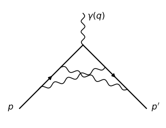
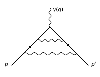
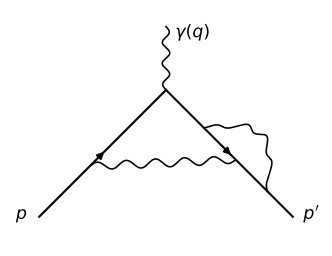
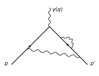
kernel, the five two-loop diagrams I, IIa, IIc, IId, IIe with their
subtractions, and the projector that turns each of them into a number —
together with a proof that their sum is the physical A2 and an
accounting of every other term the expansion generates (they all cancel,
vanish, or renormalize parameters).
The logical chain, each link derived below:
QED Lagrangian with regulators (photon mass λ, Pauli–Villars)
→ free propagators and the interaction vertex.
The quantity: ae=F2(0), with the form-factor decomposition and
the explicit Breit-frame projector proved.
The 3-point Green function and the LSZ reduction with interacting
fields: residue factors Z2, amputation by full propagators,
why external-leg diagrams (IIb/IIf) drop out.
Gell-Mann–Low formula (proved in the QFT section) + Dyson series +
Wick’s theorem (proved here, with the fermion sign rules)
→ the completely systematic algebraic expansion.
The expansion executed at orders e1, e3, e5: every single
contraction enumerated and classified (mechanically verified by
code/wick_enum.py).
The loop-integration toolkit derived: Feynman parameters, the shift,
Wick rotation, the master integral table of code/loops.py, angular
averages, Pauli–Villars.
The one-loop building blocks derived: the massive-photon vertex
(kernel K), the self-energy Σ, the vacuum polarization
Π^ and its spectral function ρ(t), the one-loop vertex
parts Λν with their Feynman-parameter denominators.
The five raw two-loop integrals written out explicitly.
Renormalization: the on-shell counterterms, the Ward identity
Z1=Z2, and the assembly theorem: the
Karplus–Kroll-subtracted diagrams of the NLO section sum exactly to
the ab-initio ae∣∣α2.
A note on terminology, since the question arises naturally: the
“systematic algebraic expansion” has two distinct steps. Expanding the
time-ordered exponential S=Texp(i∫L1) in powers of e
is the Dyson series (an ordinary Taylor expansion under the
T-symbol). Converting each resulting vacuum expectation value of a
T-product of free fields into a sum of products of propagators is
Wick’s theorem. Feynman diagrams are nothing but the bookkeeping of
the second step: one diagram per class of complete contractions. Both
steps are carried out explicitly below.
We work in the conventions of the QED and LO sections: metric
(+,−,−,−), ℏ=c=1, Dirac representation for γμ,
electron charge e (only e2=4πα ever appears). The
Lagrangian density, including the two regulators used by
Karplus–Kroll/Petermann and by all our computations, is
The last term is the interaction L1=−eψˉ/Aψ
that follows from gauge coupling (QED section); in the Dyson series
each factor iL1 produces the vertex factor
−ieγμ. Strictly the Lagrangian coupling is the bare
charge e0; the distinction (e02=e2[1−Π(0)],
§3.3) matters only in the charge-renormalization bookkeeping of
§3.3/§9, so we write e throughout and reinstate e0 exactly
there.
λ is the photon mass, the infrared regulator. Together
with the Feynman gauge-fixing term −21(∂A)2 it gives
the photon propagator its simple −igμν numerator (derived
below). This defines the IR regularization scheme of the 1950s
papers: photon propagator −igμν/(k2−λ2) everywhere,
λ→0 at the end. (A genuine Proca photon would carry an
extra kμkν/λ2 term; by the collapse lemma of §2.4 such
longitudinal pieces only produce γμ-structures, i.e. they
change F1-type contact terms, and the λ→0 limit of the
total F2 is prescription independent. All per-diagram values in
the NLO section refer to the −igμν/(k2−λ2)
prescription.)
m0=m−δm is the bare mass. We expand around the
physical mass m:
so propagators carry m and the counterterm generates an extra
two-point vertex +iδm (one insertion is order α,
exactly what is needed at two loops). The on-shell condition fixing
δm is derived in §4.2.
Ultraviolet regularization is Pauli–Villars, implemented at the
level of the single logarithmically divergent master integral (§6.5):
every log divergence is carried as the explicit symbol
LUV=logΛ2+const, and every F2 below must be
(and is, assertedly) free of LUV. For the fermion loop of the
vacuum polarization the PV subtraction must be gauge invariant
(two-mass PV); §7.3 explains where this matters and why the final
answer is unambiguous.
For the photon we need the propagator that follows from our quadratic
Lagrangian (mass term plus Feynman gauge fixing). Integrating by parts
(dropping total derivatives, which do not change the action),
Each of the four components of Aμ is a free scalar of mass
λ (with a sign from the metric for the spatial ones), so the
propagator is the inverse of the operator in brackets with the causal
iϵ, i.e. in momentum space −gμν(k2−λ2)
inverted times i:
As in the LO section, the electron scatters off a fixed classical
potential Aμcl; to first order in the potential and to
all orders in the radiative corrections the amplitude is
and the anomalous moment is ae=F2(0) where F2 is defined by the
decomposition of Γμ derived next. The connection between
F1,2(0) and the g-factor (g=2(F1+F2), Born-level matching
to −μ⋅B) was derived in full in the LO
section and is not repeated.
Claim. For on-shell spinors (/pu(p)=mu(p),
uˉ(p′)/p′=muˉ(p′), p2=p′2=m2) and a
parity-conserving theory, the most general vertex satisfying current
conservation is
Step 1 — basis.Γμ is a 4×4 matrix carrying one
Lorentz index, built from γμ, p, p′, g, and (by parity
conservation, no γ5 or ϵ-tensor) nothing else. Any
product of /p's and /p′'s sandwiched between the
on-shell spinors collapses: commute /p to the right
(/p→m) and /p′ to the left
(/p′→m) using
/a/b=2a⋅b−/b/a; each
commutation only produces scalars p⋅p′=m2−q2/2. The
sandwiched vertex therefore reduces to
with scalar functions A,B,C of q2 (the only invariant). Structures
σμνqν and σμνPν are not extra: writing
iσμνaν=−γμ/a+aμ=/aγμ−aμ
(direct consequence of σμν=i(γμγν−gμν)),
(The first line: uˉ′(−γμ/q+qμ)u with
/qu=(/p′−/p)u=/p′u−mu and
γμ/p′=2p′μ−/p′γμ, then
uˉ′/p′=muˉ′; both identities are verified
numerically below.)
Step 2 — current conservation. The Ward–Takahashi identity (derived
ab initio in §4.3) gives qμuˉ′Γμu=0 on shell.
Now q⋅P=p′2−p2=0 and
uˉ′/qu=(m−m)uˉ′u=0 hold identically, so
transversality forces q2C(q2)=0, i.e. C≡0.
Step 3 — repackaging. Use the Gordon identity to trade Pμ for
γμ and iσμνqν:
(μ,s′,s)=(1,0,1): with
γ0γ1=(0σ1σ10)
and σ1ξ1=ξ0:
uˉ′γ1u=u′†γ0γ1u=−2wξ0†σ1ξ1=−2w; and
2miσ13q3=−mwγ1γ3 with
γ1γ3=iσ212×2blocks,
iσ2ξ1=ξ0, gives
−mw[(E+m)−E+mw2]=−2w.
— the μ=1 flip sandwich alone measures only the magnetic
combination F1+F2, which is why it must be paired with the μ=0
sandwich. Solving the 2×2 linear system:
which is precisely the projection formula quoted and used in the NLO
section (code/g2_iid.py validates it on the LO diagram). Everything
above is verified symbolically:
>>> import sys; sys.path.insert(0, 'code')
>>> from sympy import symbols, simplify
>>> from dirac import formfactor_basis
>>> m, w = symbols("m w", positive=True)
>>> [simplify(b) for b in formfactor_basis(m, w, 0, 0, 0)]
[2*m, -2*w**2/m]
>>> [simplify(b) for b in formfactor_basis(m, w, 1, 0, 1)]
[-2*w, -2*w]
2.4 The collapse lemma (longitudinal photon pieces)¶
For later use (gauge/regulator independence, Ward manipulations): for
any internal-photon momentum k attached to the electron line next to
an on-shell end,
Iterating such telescoping steps, a kμkν numerator on an
internal photon collapses the two adjacent propagator chains and leaves
only γμ-type (i.e. F1-type) structures. Both identities
are checked numerically in the pipeline conventions (they are two-line
consequences of (/p−m)u(p)=0).
3. Green functions, LSZ with interacting fields, and amputation¶
with the external legs stripped by the reduction rules of the QFT
section. Those rules were derived there with free-field residues; at
two loops we need the refinement that the interacting field creates the
physical one-electron state with amplitude
Z2 is defined by this equation. Repeating the free-field computation
of the propagator with this matrix element (insert a complete set of
states into ⟨Tψψˉ⟩; the one-particle
contribution reproduces the free two-point integral times Z2, with
the physical mass m in the exponentials; multi-particle states start
at the cut p2≥(m+λ)2) gives the exact two-point function
near its pole:
Consequently the correct reduction rule for each external fermion leg is
the QFT-section rule divided by Z2 (the free rule assumed unit
amplitude), with m the physical mass.
Let −iΣ(/p) denote the sum of all one-particle-
irreducible (1PI) self-energy insertions (plus the +iδm
counterterm vertex, so Σeff=Σ−δm; we write
Σ for Σeff from here on). Summing the geometric
series of blobs strung on free propagators,
Identically for the photon: with iΠμν(q)=(q2gμν−qμqν)iΠ(q2) the 1PI photon self-energy
(transversality is derived in §7.3), the dressed propagator sums to
(displayed at λ=0; the qμqν terms never contribute by
§2.4 and the Ward identity).
3.3 Factorized form of G~μ and the S-matrix vertex¶
Every connected diagram of G~μ decomposes uniquely as
(blobs on the p leg) ⊗ (blobs on the p′ leg) ⊗ (vacuum-polarization
chain on the photon leg) ⊗ (core vertex 1PI in all three legs). This is
not an assumption: at the orders we need it is verified term by term
by the complete enumeration of §5 — every contraction lands in exactly
one class (the odd-loop class V would be additional core diagrams, but
it cancels pairwise by Furry’s theorem, §5). Therefore, exactly,
(using (/p′−m)(/p′+m)=p′2−m2; the regular part
of S~′ is killed by (/p′−m)u=0), and similarly
Z2u(p) on the incoming side. The photon leg is the external
potential; its propagator and 1/(1−Π) dressing combine with the
charge as follows. On-shell charge renormalization defines
Three structural conclusions, each an exact statement about classes of
diagrams:
External-leg self-energies (KK classes IIb, IIf and all their
two-loop variants) never enter the vertex. They are part of
S~′(p(′)) and are consumed by the reduction, which
leaves only the number Z2 per leg — total factor Z2.
Vacuum-polarization chains on the external-potential line (KK
classes III and IV) are the factor 1/(1−Π(q2)). After charge
renormalization they contribute Fiblob(q2)Π^(q2);
since Π^(0)=0 and all Fiblob are finite at
q2=0, they contribute nothing to ae=F2(0): pure
charge renormalization.
This is the master ab-initio formula. By the Ward identity (§4.3)
δZ2=−δF1(0), so the second term is exactly the
“vertex renormalization cross term
−δF1(0)⋅2πα” of the NLO section.
with here $\mathcal{L}_1 = -e\bar\psi\slashed{A}\psi
\delta m,\bar\psi\psi(allfieldsinteraction−picturefreefields).Taylor−expandingtheexponentialundertheTsymbol(legitimatebecauseeverythinginsideoneT−productcommutesbyconstruction)givestheorder−e^n$ term of the 3-point function:
plus, at each order in α, the terms with δm insertions.
Only odd n survives (the photon fields must pair up: n vertex
photons + 1 external photon must be even). The vacuum diagrams generated
simultaneously in ⟨0∣S∣0⟩ cancel: any complete contraction
factorizes uniquely into its externals-connected part (say n1
vertices) and its vacuum part (n2=n−n1 vertices); summing over
which labeled vertices go where turns 1/n!(n1n) into
n1!1n2!1, so the numerator factorizes as
(no-vacuum series) × ⟨0∣S∣0⟩ and the denominator removes
the second factor exactly.
Definitions. For a free field ϕ=ϕ++ϕ−
(ϕ+ annihilates, ϕ− creates), the normal productN{⋯} puts all ϕ− left of all ϕ+, with a factor
(−1) for each transposition of two fermionic fields performed in the
rearrangement. The contraction of two fields is the c-number
Because [ϕ+(x),ϕ−(y)]∓ is a c-number for free fields,
the contraction is a c-number, and taking ⟨0∣⋅∣0⟩
(normal products of one or more fields have zero vacuum expectation
value) shows it equals the propagator:
ψa(x)ψˉb(y)=Sab(x−y),
Aμ(x)Aν(y)=Dμν(x−y), and
ψψ=ψˉψˉ=0.
where the sign of each term is the parity of the permutation that
brings every contracted pair into adjacent order (fermions
anticommute, bosons commute, in this counting).
Proof (induction in n). For n=2 this is the definition of the
contraction. Assume the statement for n−1 fields. Both sides change
by the same graded sign under any permutation of the fields (that is
how T, N, and the pair-adjacency sign are all defined), so we may
relabel such that t1 is the earliest time; then
T{ϕ1⋯ϕn}=T{ϕ2⋯ϕn}ϕ1, and by the
induction hypothesis the right-hand side is [the signed contraction sum
of ϕ2⋯ϕn inside normal products] ×ϕ1.
Split ϕ1=ϕ1++ϕ1−. The annihilation part ϕ1+
already stands in normal position at the far right. The creation part
ϕ1− must be moved to the far left; each transposition past the
annihilation part ϕk+ of an uncontracted field produces the
graded commutator [ϕk+,ϕ1−]∓ — a c-number equal to
⟨0∣ϕkϕ1∣0⟩=⟨0∣Tϕkϕ1∣0⟩
(since tk≥t1), i.e. exactly the contraction
ϕkϕ1 — while the transposition signs accumulate
into precisely the pair-adjacency sign of that new contraction.
Collecting the terms with and without the new contraction reproduces
the claimed sum for n fields. ■
Taking the vacuum expectation value kills every term with uncontracted
fields:
Open fermion line. In the canonical operator order
ψoutψˉin(ψˉ1ψ1)(ψˉ2ψ2)⋯ every contraction whose
fermion pairs form only an open line from ψˉin to
ψout has total sign +1.
Closed fermion loop. Each closed loop contributes one factor
(−1) and a Dirac trace. Derivation on the shortest case, the
two-vertex loop
⟨(ψˉΓ(1)ψ)x(ψˉΓ(2)ψ)y⟩:
the only contraction is
ψˉa(x)Γab(1)ψb(x)ψˉc(y)Γcd(2)ψd(y) with
ψb(x)ψˉc(y)=Sbc(x−y) and the pair
(ψˉa,ψd) contracted in reversed order: bringing
ψd in front of ψˉa costs the T-reordering sign
⟨Tψˉaψd⟩=−Sda(y−x), so the term equals
−Sda(y−x)Γab(1)Sbc(x−y)Γcd(2)=−tr[Γ(1)S(x−y)Γ(2)S(y−x)].
The general loop works identically (one reversed pair per loop).
Both rules — and nothing else about signs — are verified for every
single contraction through two loops by code/wick_enum.py (§5),
which computes each term’s permutation sign explicitly and asserts
sign=(−1)#closed loops.
The fermion equation of motion from §1,
(i/∂−m0−e/A)ψ=0 and its conjugate,
give current conservation as an operator equation regardless of the
photon mass (the /A and mass terms cancel between the pair):
Fourier transforming (conventions of the QFT section) and amputating
the two fermion legs with full propagators turns this into the
momentum-space Ward–Takahashi identity for the proper vertex; the
overall normalization is fixed by the tree-level check
(Γμ=γμ, S~′−1=−i(/p−m)):
On shell both sides sandwiched with uˉ(p′)…u(p)
vanish: qμuˉ′Γμu=0 (used in §2.2).
q→0: write Σ(/p)=A(p2)+B(p2)/p
and expand the identity to first order in q; sandwiching and using
the q=0 Gordon identity uˉpμu=muˉγμu
to convert the Pμ-structures,
(The identity holds to all orders; we only need it at order
α.) In particular F1S(0)=Z2F1(0)=1 exactly: the
charge is not renormalized by the vertex, and the LO section’s
renormalization condition “F1(0)=1 to all orders” is automatic.
Applying Wick’s theorem to the Dyson term of §4.1 and Fourier
transforming every propagator, each ∫d4xi produces
(2π)4δ(4)(∑kin) at vertex i; one delta
survives as overall momentum conservation and the remaining momentum
integrals are the loop integrals. The dictionary (all derived above):
element
factor
vertex
−ieγμ
mass counterterm vertex
+iδm
fermion propagator
i(/k+m)/(k2−m2+iϵ)
photon propagator
−igμν/(k2−λ2+iϵ)
closed fermion loop
(−1)×tr[⋯], ∫(2π)4d4l
loop momentum
∫(2π)4d4k
Combinatorial weight. For a fixed topology with no vertex-exchange
automorphism, the n! assignments of the labeled integration variables
x1…xn to the n vertex positions give identical integrals and
cancel the Dyson 1/n! exactly: every distinct diagram enters with
weight one. This is not left as folklore: code/wick_enum.py counts
the contractions of every topology at n=1,3,5 and verifies that
each single-topology class appears exactly n! times per orientation
or mirror copy.
all perfect matchings of the n+1 photon fields times all (n+1)!
pairings of ψ’s with ψˉ’s, then classifies the topology
and computes the fermion sign of each term. Output
(pixi run python code/wick_enum.py):
order e^1: 2 complete contractions (1 photon matchings x 2! fermion pairings)
topology class count /n! sign
tadpole loop tr[gamma S(0)] = 0 1 1 -1
tree vertex gamma^mu 1 1 +1
total 2 2
all signs equal (-1)^(# closed fermion loops): OK
order e^3: 72 complete contractions (3 photon matchings x 4! fermion pairings)
topology class count /n! sign
tadpole loop tr[gamma S(0)] = 0 39 - +1/-1
external-leg corrections only (tree vertex) 12 2 +1
III: VP on the external-potential line x tree vertex 6 1 -1
LO one-loop vertex correction 6 1 +1
forward line x (rest): no scattering / disconnected 6 1 -1
disconnected (vacuum bubble or detached blob) 3 - -1
total 72 12
all signs equal (-1)^(# closed fermion loops): OK
order e^5: 10800 complete contractions (15 photon matchings x 6! fermion pairings)
topology class count /n! sign
tadpole loop tr[gamma S(0)] = 0 6165 - +1/-1
external-leg corrections only (tree vertex) 840 7 +1
forward line x (rest): no scattering / disconnected 660 - +1/-1
disconnected (vacuum bubble or detached blob) 495 - +1/-1
V: odd fermion loop (Furry pair, cancels) 480 4 -1
III: two-loop VP blob on the external-potential line 360 3 -1
III: VP on the external-potential line x leg SE 240 2 -1
IIb/IIf: LO vertex x self-energy on an external leg 240 2 +1
IIc: corner, vertex part at an internal vertex (+ mirror) 240 2 +1
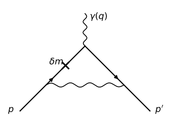
IId: self-energy on an internal line (+ mirror) 240 2 +1
external-leg SE with VP insertion 240 2 -1
I: crossed ladder 120 1 +1
III: VP on the external-potential line x vertex corr. 120 1 -1
IIa: ladder (vertex part at the external vertex) 120 1 +1
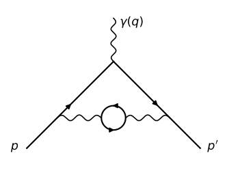
IIe: vacuum polarization in the internal photon 120 1 -1
IV: iterated one-loop VP chain on the external-potential line 120 1 +1
total 10800 90
all signs equal (-1)^(# closed fermion loops): OK
The classification logic is elementary once the fermion chain is laid
out: order the open-line vertices from the incoming electron as
v1…vk, note where the external photon attaches, and note which
pairs the two internal photons connect; closed fermion cycles are the
loops. Reading the n=5 table row by row gives the complete fate map of
the two-loop expansion:
Kept (the 1PI vertex cores):
I — crossed ladder (weight 1): both photons span the external
vertex and cross;
IIa — ladder (weight 1): both span, nested — a one-loop vertex
subgraph at the external vertex;
IIc — corner (weight 2 = the two mirror reflections): outer
photon spans the external vertex, inner photon spans one of its
internal attachment points;
IId (weight 2 = mirrors): self-energy subgraph on one of the two
internal fermion propagators of the LO diagram;
IIe (weight 1): fermion loop (with its -1 and trace) inserted
in the internal photon.
The mirror image of a diagram (reflect through the external vertex,
i.e. read the string backwards and exchange p↔p′)
has the same F2(0) — the Breit-frame projection of §2.3 is
symmetric under w→−w combined with the relabeling — so the NLO
section computes one orientation of IIc and IId and doubles it.
The five distinct contributions are exactly Karplus–Kroll’s.
External-leg classes (IIb/IIf, the seven “external-leg-only”
topologies, “leg SE with VP insertion”): all live inside
S~′(p) or S~′(p′) and are consumed by LSZ (§3.3),
leaving the single factor Z2. No integral to compute, ever.
External-potential classes III and IV (VP blob, chain, or blob ×
line correction on the q line): the 1/(1−Π(q2)) dressing;
after on-shell charge renormalization they contribute
Π^(0)=0 to F2(0) (§3.3). The weight 3 of the two-loop
blob row is the three standard two-loop photon-self-energy graphs;
none of this is ever integrated either.
Class V — odd fermion loops (a fermion triangle attached to the
potential and by two photons to the electron line, or attached once
to the line and closed on itself by a photon with the potential on
the line): vanish pairwise by Furry’s theorem, proved as
follows. The charge
conjugation matrix C=iγ2γ0 satisfies
C−1γμC=−(γμ)T, hence
C−1S~(k)C=S~(−k)T. Insert CC−1 between all
factors of an ℓ-vertex loop trace and transpose:
which after renaming loop momenta is exactly the trace of the
orientation-reversed loop. The enumeration confirms that odd loops
come in orientation pairs (the count 480=2 subclasses × an
orientation pair ×5!); for odd ℓ each pair sums to
zero. The ℓ=1 tadpole is
its own reversal and vanishes identically,
tr[γμS~(l)]∝lμ→0 by symmetric
integration — consistent with the same C argument.
Disconnected / forward classes: cancelled by the
⟨0∣S∣0⟩ denominator (§4.1) or proportional to
no-scattering δ-functions; they never reach Γμ.
δm counterterm terms (order e3×δm, not in
the table): insertions on the two internal lines pair with IId
(§8.4); insertions on external legs join the external-leg class and
drop with it.
At order e3 the same table shows the familiar one-loop result: the
proper vertex is the single LO diagram (weight 1) — everything else is
legs, potential dressing, tadpoles, or vacuum.
Induction step: assume the (n−1)-denominator formula; apply the base
case to combine the (n−1)-fold denominator with An, then rescale
the parameters — this yields
by expanding both sides (k2 coefficients match; linear terms fix
s; the rest is Δ). The shift k=ℓ+s has unit Jacobian.
feynman_shift does exactly this and verifies the reduction to
ℓ2−Δ symbolically.
For Δ>0 the integrand poles in the ℓ0 plane sit at
ℓ0=±(ℓ2+Δ−iϵ)
— second and fourth quadrants. The closed contour (real axis, arc,
imaginary axis, arc) therefore encloses no pole, the arcs vanish for
convergent integrands, and
(the Beta integral, by the substitution t=Δv/(1−v)).
Assembling with the Wick-rotation factor i(−1)a+n from
(ℓ2)a=(−1)a(ℓE2)a and
(ℓ2−Δ)n=(−1)n(ℓE2+Δ)n:
For n−a−2=0 subtract the identical integrand with
Δ→ΔΛ (Δ shifted by the regulator mass
Λ2→∞). The difference is convergent and elementary:
differentiating in Δ lands on the convergent case of §6.4,
with LUV≡logΛ2+const. The additive
constant (and the difference between subtracting at the integral level
and the historical propagator-level PV) is a scheme constant insideLUV; since LUV cancels identically in every renormalized
quantity below (asserted by the scripts), it never matters.
After the shift the denominator depends on ℓ2 only, so odd
powers of ℓ integrate to zero and even ones can be replaced by
their rotational averages (Euclidean rotation invariance after §6.3).
By Lorentz covariance ⟨ℓμℓν⟩=cgμνℓ2;
tracing with gμν gives 4c=1:
the rank-4 coefficient fixed by the double trace (16+4+4=24). The
general even rank ((ℓ2)n/(2n(n+1)!)∑matchings∏g) is what symmetrize implements; ranks 2 and 4 are
all the diagrams below need.
odd traces vanishing. (The pipeline needs none of these as rules —
it multiplies explicit 4×4 matrices — but they are what make the
hand-derivations below short.)
7.1 The LO vertex with a massive photon → the kernel K(t)¶
From the n=3 row of §5, the proper vertex at one loop is the single
diagram with the photon spanning the external vertex. Its Wick
contraction, Fourier transformed with the rules of §4.4 (routing as in
the LO section and code/g2_lo_trace.py: fermion momenta k, k′=k+q,
photon k−p):
the prefactor being (−ie)2ii(−i)=−ie2 from two vertices,
two fermion propagators and one photon propagator (the gνρ of
the photon contracts the two vertex indices into
γν⋯γν). The iϵ’s are kept implicit from
here on. Using §6.7 the numerator reduces exactly as in the LO section:
Feynman parameters (§6.1) with x on the photon, y on k′, z on
k, x=1−y−z; the shift (§6.2) with ax=p, ay=−q,
az=0 gives s=xp−yq and (using p⋅q=−q2/2,
x+y+z=1)
which at q2=0 is exactly the Delta printed by
pixi run lo-trace-sympy. (The LO section’s variables put the
parameter z on the photon; the two labelings are related by
zLO=1−y−z and give identical integrals.) The numerator with
k=ℓ+s is expanded, averaged (§6.6), and integrated with the
master table (§6.4–6.5); the F2 projection (§2.3) of the result —
performed symbolically by the pipeline, every intermediate checked —
gives at q2=0, m=1:
is free of LUV: the three LUV coefficients are
(4m−2u/k), −(4m−2um), and +2u(/k−m), which sum
to zero pointwise in u — the cancellation asserted by the script.
ΣR splits into a rational part and a
log(Din(k2)/Din(m2)) part; the log is
rationalized with the elementary identity (differentiate
log[Y+ξ(X−Y)] and integrate back)
which, applied to X=a−bk2, Y=a−bm2, produces the factor
(k2−m2) that cancels one power of the doubled propagator and leaves
an ordinary propagator of squared mass
C=m2+(a−bm2)/(ξb)>m2 — the NLO section’s ξ-trick,
here derived.
7.3 The vacuum polarization Π^ and its spectral function¶
The fermion-loop contraction with its (−1) and trace (§4.2):
Transversality. The Ward–Takahashi argument of §4.3 applied to
⟨Tjμ(z)jν(y)⟩ (the equal-time commutator
[j0,jν] vanishes up to Schwinger terms that a gauge-invariant
regulator cancels) gives qμΠμν=0, i.e.
Maintaining this in regularization is exactly why the fermion loop
needs gauge-invariant Pauli–Villars (two heavy masses Mi with
coefficients satisfying ∑ci=0, ∑ciMi2=0, which
remove the quadratically divergent non-transverse polynomial). Granted
transversality, Π(q2) can be read off from the qμqν
coefficient, which is only log divergent and hence unambiguous:
Feynman parameter x, shift l=ℓ+xq,
— finite, with Π^(0)=0: the once-subtracted (on-shell charge
renormalized) vacuum polarization of §3.3.
Spectral (dispersion) form.Π^(q2)/q2 is analytic in the
q2 plane cut along [4m2,∞) (the log argument
m2−x(1−x)q2 can vanish only for q2≥4m2 since
x(1−x)≤41) and falls off like log(−q2)/q2; the Cauchy
formula on a contour hugging the cut plus a large circle (whose
contribution vanishes) gives the unsubtracted dispersion relation
The imaginary part is elementary: with q2=t+iϵ the argument
m2−x(1−x)t becomes negative for
x∈(x−,x+), x±=21(1±β),
β=1−4m2/t, where the log acquires −iπ; hence
Feynman parameters u on the (p′−k−k2) line, v on the (p′−k2)
line, 1−u−v on the photon. The shift formula (§6.2) with
au=p′−k, av=p′, aph=0 gives
s=(u+v)p′−uk and (using p′2=m2; verified symbolically)
D0 is the LO Δ (at q2=0) with z=u+v — the origin of
the “D0” in the NLO section. After the shift and angular average the
numerator has an ℓ2 part and an ℓ-free part Nν. The
ℓ2 part is proportional to γν with a constant
coefficient: by §6.6 and §6.7,
γρ/ℓγν/ℓγρ→4ℓ2γργαγνγαγρ=4ℓ2γρ(−2γν)γρ=ℓ2γν.
Applying the master integrals (n=3: the ℓ0 part is finite, the
ℓ2 part log divergent):
with Pν(k)=−16π2e2Nν(k) — exactly the
Λν structure of the NLO section
(c=e2/8π2), whose explicit Nν the pipeline
(pixi run iic-sympy) constructs as matrices.
KK “reduced diagram” subtraction. Setting k=0 and q=0
(both electron legs on shell) in the integrand turns it into the
(u,v)-integrand of the one-loop F1(0), i.e. of
δF1(0;λ) (§7.1) — the vertex subgraph collapses to
γν×scalar by §2.2 at q=0. Define the pointwise
subtraction
ΛRν(k)≡Λν(k)−[D0La(u,v)+8π2e2(LUV−logD0)]γνunder the (u,v) integral,∫∫[⋯]dudv=δF1(0;λ)γν.
LUV cancels pointwise (same constant c), so ΛRν
is UV finite before any outer integration — this is the subtraction
Karplus–Kroll perform “within the diagram”, and the reason the NLO
section’s IIa and IIc integrands are finite. The log-ratio
log(Δin/D0) is rationalized with the same ξ-identity
as in §7.2.
IIa version (both electron legs internal, p−k and p′−k; the
subgraph dresses the external vertex, so the open index is μ and
the external momentum q enters the loop):
These are the order-e5 1PI cores of §5, written with the rules of
§4.4. Overall factors: four internal vertices (−ie)4=e4; the
external vertex’s −ie is factored out into the definition of
Γμ as always. Momentum routings match the pipeline scripts
exactly. All expressions are for the vertex matrix
δΓμ; the number that the NLO section calls
μX is its projection (§2.3) in units (α/π)2,
including the stated subtraction and mirror factor.
Photons ka (vertices 1,4 counting from the incoming electron) and
kb (vertices 2,5), external photon at vertex 3. Four fermion
propagators (i4=1), two photon propagators ((−i)2=−1):
(Read the numerator right to left along the electron line: emit ka
(γν), emit kb (γρ), absorb q (γμ),
absorb ka (γν), absorb kb (γρ) — the
crossing is the index pattern
ν…ρ…μ…ν…ρ.) No subdiagram is a
vertex or self-energy part, so there is nothing to subtract; the
ka- and kb-subintegrals are separately convergent by power
counting (each one-loop subintegral sees one photon and three fermion
propagators: superficial degree 4−2−3=−1), the overall degree is
8−4−4=0, and the log lives in
the γμ (F1) structure only — the F2 projection is UV
finite as it stands, and IR finite (no logλ) in the KK scheme.
Outer photon k (vertices 1,5), inner photon k2 (vertices 2,4)
nested around the external vertex 3 — i.e. the inner vertex part
ΛIIaμ(k) of §7.4 inserted at the external vertex of
an LO-type outer loop:
KK subtraction: replace ΛIIaμ→ΛIIaμ−L(u,v)γμ pointwise (§7.4); the
subtracted piece, −L(u,v)×(LO diagram integrand), factorizes and
integrates to −δF1(0;λ)⋅F2(2)(0). The ladder is
its own mirror image: no doubling.
This — with §7.4’s ΔinIIa — is the complete
defining integral for the NLO section’s TODO diagram IIa
(code/g2_iia.py implements exactly this construction: the three
pieces (a) Pμ/Δin, (b) −L/D0, (c) the
log(Δin/D0) term via the ξ-identity).
Outer photon k (vertices 1,4), inner photon k2 (vertices 3,5)
around the outer photon’s p′-side attachment, external photon at
vertex 2 — i.e. Λν(k) of §7.4 inserted at an internal
vertex:
(note the outer photon propagator carries k2 itself in this
routing, as in code/g2_iic.py). KK subtraction: the same
pointwise −L(u,v)γν; the subtracted cross term again
integrates to −δF1(0;λ)F2(2)(0) — this is the NLO
section’s piece (b), which factorizes and carries the entire
−logλ of IIc. Mirror: the reflected diagram (subgraph at
the p-side attachment) contributes equally: factor 2.
i.e. the sum of the NLO section’s pieces (a), (b), (c), whose
integrands fa,fb,fc already include this factor 2.
8.4 Diagram IId (self-energy insertion) + mass counterterm¶
The raw insertion (routing of code/g2_iid.py: fermion momenta k,
k′=k+q, photon k−p; the SE sits on the k line, giving the
doubled propagator; five fermion propagators i5=i, two photons
(−i)2=−1, vertices e4):
with Σloop the integral of §7.2 (substituting it makes
this the explicit double integral; the collected prefactor is
(−ie)2i3(−i)×(−iΣ-blob)=−ie2Σ from two
outer vertices, three fermion and one photon propagator, and the
blob). The δm counterterm diagram
is the same string with −iΣloop→+iδm, i.e. it
replaces Σloop→Σloop−δm. The KK
(= full on-shell) scheme also removes the δZ2 part:
δΓIIdμ=same string with ΣR(k)=Σloop(k)−δm−(/k−m)δZ2.
(prefactor (−ie)2i2=e2 from the two outer vertices and two
fermion propagators; the photon factors are displayed). Renormalization
replaces Π→Π^ (the Π(0) part is the charge
renormalization of the LO diagram, §3.3/§9). Because
Π^(kγ2)∼kγ2 as kγ2→0, the diagram
is IR finite and λ can be set to zero here. Using
transversality and the spectral representation (§7.3),
kγ2−igαρi(kγ2gρσ−kγρkγσ)Π^(kγ2)kγ2−igσβ=−igαβkγ2Π^(kγ2)+(kγαkγβterms⇒F1-structures only, Sec. 2.4)
i.e. diagram IIe = the LO diagram with a photon of mass2t,
folded with ρ(t). Since §7.1 gives that diagram’s F2(0) as
(α/π)K(t)linearly in the photon propagator,
Collecting §3.3, §5, §7 and §8, with everything expressed in the
physical m (via δm) and physical α (via Π^), the
ab-initio order-α2 anomalous moment is
every term a fully specified integral. The NLO section instead
computes the KK-subtracted per-diagram contributions (write aX
for the absolute F2(0) contribution; the NLO section’s numbers are
μX=aX/(α/π)2):
(§8.2–8.4: the pointwise vertex subtractions integrate to
δF1(0)F2(2) per insertion, and the on-shell δZ2
subtraction collapses to δZ2F2(2) per line). Summing and
comparing with the master formula:
This is the precise sense in which the five scheme-dependent
per-diagram integrals of the NLO section — three vertex subtractions
but only one net LSZ cross term, reconciled by Z1=Z2 — sum to
the scheme-independent A2, and it derives the NLO section’s
renormalization bookkeeping (its “vertex renormalization cross term”
and “caveat on per-diagram comparisons”) rather than assuming it. The
infrared side is organized the same way: the logλ of
δF1(0;λ) enters IIa and IIc through their subtractions
and δZ2(λ) enters IId through its subtraction; the NLO
section verifies explicitly that only the advertised
∓21log(λ2/m2) of IIc/IId survives and cancels in the
sum.
The Green function
⟨Ω∣TψAμψˉ∣Ω⟩, expanded by
Gell-Mann–Low + Dyson + Wick, contains at order e5 exactly 10800
complete contractions in 16 topology classes with total weight
10800/5!=90 (code/wick_enum.py). Of these:
disconnected, forward, and tadpole classes are zero or cancel
against ⟨0∣S∣0⟩;
class V vanishes by Furry’s theorem (proved via charge conjugation);
external-leg classes are absorbed by LSZ into Z2;
external-potential classes III/IV are absorbed by on-shell charge
renormalization (Π^(0)=0);
the remaining five 1PI cores — with the on-shell/KK subtractions
derived in §7–§9 and the projector of §2.3 — are the integrals
μI,μIIa,μIIc,μIId,μIIe, and their sum is exactly A2.
Their evaluation — Feynman-parameter reduction, Fortran quadrature,
and sequential analytic integration — is the subject of the NLO
section: the massive-photon kernel K(t) (§7.1 here = Stage 0 there),
μIIe (§8.5 = its dispersion integral), μIId
(§7.2/§8.4 = its frat/flog), μIIc
(§7.4/§8.3 = its pieces (a),(b),(c)), μIIa (§7.4/§8.2, same
machinery, no mirror), and μI (§8.1, the genuine two-loop
integral). Nothing in that section’s list of integrals falls outside
this derivation, and nothing derived here requires an integral not
listed there.